A Markov chain is a sequence of random variables whose current state depends only on the previous one and is independent of all states before it. This condition is known as the memoryless or Markov property. Their applications span many areas of statistics, including parameter inference and statistical modelling.
The Markov property implies that the current state is a random variable whose possible values are described by a probability density dependent on the previous state. Being sequential, Markov chains are usually thought to progress with time, with updates occurring at discrete or continuous intervals. The state space of a Markov chain, the possible values of the random variables, can be either multi- or univariate and be discrete or continuous. Here we introduce both discrete and continuous state-space Markov chains with an example of both. The discussion is limited to discrete-time Markov chains, that iterate at fixed time intervals but continuous-time extensions exist. It is assumed that the reader is familiar with conscepts in statistics such random variables and probability density functions.
Discrete state-space Markov chain
Let ${X_t : t=0,1,2,\dots}$ be a sequence of random variables which form a discrete-time, discrete state-space, stochastic process. That is, a Markov chain which updates at discrete and fixed time increments and whose value can be a finite number of possibilities. Let the possible bales of $X_t$ be denoted by $\mathcal{S}={S_1, S_2, \dots, S_m}$ i.e. $X_t\in\mathcal{S}$ for all $t=0,1,2,\dots$. Assume that the probability of moving between any two states, $S_i, S_j\in\mathcal{S}$, is known, independent of time and denoted $p_{ij}$ such that $\text{Pr}\left(X_t = S_j | X_{t-1} = S_i\right) = p_{ij}$, for all t$\geq1$ and for all $1\leq i,j \leq m$.
Given that at time index $t$ the previous state is $X_{t-1} = S_i$, the transition probabilities ${p_{i1}, p_{i2}, \dots, p_{im}}$ form a probability mass function (PMF) describing the distribution of $X_{t}$. The system can, therefore, be forward-simulated with a known starting condition by recursively sampling from the appropriate PMF. Although this may appear confusing, the following example will hopefully provide some clarity.
Discrete state-space example
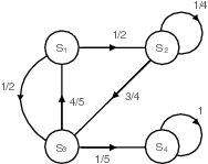
Suppose a system can be in four distinct states, ${S_1, S_2, S_3, S_4}$, with known transition probabilities, the system can be represented in a directed graph, as shown in Figure 1. Here, by inspection of the graph, it can be seen that when the system is in $S_1$, the next state can be either $S_2$ or $S_3$, with equal probability.
|
|---|
| Figure 1: Discrete state-space Markov chain. A directed graph showing the possible transitions and their probabilities of the Markov chain. The directed edges between nodes indicate a possible transition over a discrete time interval. For example, moving from $S_2$ to $S_3$, over one time increment, is possible, but not from $S_3$ to $S_2$. Each transition is associated with probability, seen adjacent to the edge connecting to nodes. |
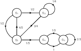
Intuitively, within the system described in Figure 1, the probability distribution of the current system state depends only on the previous state and not any state before that. It can also be seen in the directed graph that if the system reaches $S_4$, it will remain in this state indefinitely. This is an example of a stationary distribution of the Markov chain. Given an infinite amount of time, the system will reach $S_4$ with probability 1, and once it does, it can not escape. In this example, the stationary distribution has all weight associated with $S_4$ and none to the other states. Although in more complex systems, this may not be the case. For example, the system depicted in Figure 2, shows a stationary distribution split across two states; $S_4$ and $S_5$. By inspection of the directed graph, it is clear that once the system enters $S_4$, it will oscillate between $S_4$ and $S_5$ indefinitely.
|
|---|
| Figure 2: Discrete state-space Markov chain with non-singular stationary distribution. A directed graph showing the possible transitions and their probabilities of the Markov chain. The connections between nodes indicate that it is possible to transition between the two states over a discrete time interval. The arrow of these connections indicates in which direction it is possible to move. The stationary distribution of this Markov chain has equal weight associated with states $S_4$ and $S_5$ but zero weight associated with the remaining nodes. |
A stationary distribution represents the time-limiting behaviour of the system and the proportion of time the chain spends in each state as the system-time tends to infinity. If one exists, the system’s stationary distribution can be calculated analytically for discrete-time, discrete-state-space Markov chains.
As the size of the state space increases, summarising the possible transitions and their probabilities within a directed graph becomes inconvenient. Therefore, this information is often summarised in a transition matrix, whose \((i,j)\)-th element is the probability of transitioning from state \(i\) to \(j\), \(p_{ij}\). For the system described in Figure 2, the transition matrix, \(P\), is
\[ P = \begin{pmatrix} 0 & 1/2 & 1/2 & 0 & 0 \\ 0 & 1/4 & 3/4 & 0 & 0 \\ 4/5 & 0 & 0 & 1/5 & 0 \\ 0 & 0 & 0 & 0 & 1 \\ 0 & 0 & 0 & 1/3 & 2/3 \end{pmatrix}. \]
The $i$-th row of the transition matrix is the PMF of the current state if the system was previously in the $i$-th state. For example, the $3^\mathrm{rd}$ row, $\left(4/5, 0, 0, 1/5, 0 \right) $ gives probabilities 4/5 and 1/5 of being in the $1^\mathrm{st}$ and $4^\mathrm{th}$ states, respectively, and all other states having a zero probability. This is reflected in Figure 2 where the only directed edges leaving $S_3$ are to $S_1$ and $S_4$, with the appropriate weights.
Continuous state-space Markov chain
Discrete state-space Markov have a wide number of applications and are useful to gain an intuition into Markov chain behaviour. However, a number of applications require continuous state-space. For example Markov chains are a key component in Bayesian inference, where a posterior distribution is sampled from by a Markov chain. As many model parameters are continuous, they require a continuous state-space Markov chains. Continuous state-space Markov chains are also required in mathematical models where the modelling output is not appropriately approximated by discrete values, such as stochastic models of stock price or molecular concentrations during a chemical reaction.
Similarly to the discrete state-space version, the continuous state-space Markov chain possesses the Markov property. However, due to the continuous state space, the transition probabilities can no longer be expressed exactly and must be considered using transition densities. Much like the difference between discrete and continuous random variables.
Let ${X_t : t\geq 0}$ be discrete-time stochastic process, and $X_t \in \mathcal{S}$ be a continuous state-space, such as $\mathbb{R}$. The memoryless property implies that the distribution of the current state, $X_t$, depends only on the previous, $X_{t-1}$, and is independent of $X_{t-2}, X_{t-3}, \dots, X_0$. For a transition density $f$ that is $$ f\left(X_t | X_{t-1}, X_{t-2}, \dots, X_0\right) = f\left(X_t | X_{t-1}\right). $$
Continuous state-space Markov chains possess many of the same properties as their discrete counterparts. However, their transition probabilities cannot be succinctly summarised in a matrix. and they can be forward simulated. An example of a continuous state-space Markov chain is introduced here.
Continuous state-space example
Let ${X_t: t=0,1,2,\dots}$ be real-valued random variables that are sequentially updated by adding normally distributed independent random noise. That is, given an initial value $X_0=x_0$, for $t=1,2,\dots$ $$ X_t = X_{t-1} + \varepsilon_t, \ \varepsilon_t \sim \text{Norm}\left(0, \sigma^2\right), \hspace{0.5cm} \text{indep.} $$
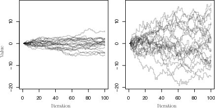
The random variables ${X_t : t=0,1,2,\dots}$ form a continuous state-space, discrete-time Markov chain, referred to as a normal random walk. Whose transition density is a normal distribution centred around the previous state, with variance $\sigma^2$. Figure 3 shows a number of realisations from this model, with varying standard deviations of the additive random noise.
|
|---|
| Figure 3: Example simulations of normal random walk. Twenty realisations from a normal random walk, with initial value $X_0=0$ (both) and standard deviations $\sigma=0.25$ (left) and $\sigma=1.0$ (right). |
As presented here, the normal random walk is univariate; however, this need not be the case, and extending the Markov chain to be multivariate is relatively straightforward.
Final remarks
Markov chains provide a useful framework for modelling random systems that evolve sequentially, especially when the next state can be described using only the current one. Whether the state space is discrete or continuous, the key idea is the same: specify how the system moves locally, then study the behaviour that emerges over time. This perspective makes Markov chains useful both as models in their own right and as computational tools, including in simulation and Bayesian inference. Further topics such as irreducibility, recurrence, convergence, and Markov chain Monte Carlo build on the same foundation introduced here.