Sampling from a finite set of weighted outcomes is a small task that appears surprisingly often in simulation, stochastic modelling, and Monte Carlo methods. In this post we build a compact C++ function for drawing from a discrete distribution, then compare its behaviour with std::discrete_distribution.
We will briefly discuss how to sample a discrete random variable in theory and practice, before constructing our own algorithm and comparing its performance to the std::discrete_distribution in the C++ standard library. Many hand-coded discrete samplers have been proposed, but often these are unnecessarily clunky and, consequently, slow.
The sampler proposed here is a function, designed to take an std::vector input representing the weights of the possible outcomes and return an std::size_t value indicating the randomly sampled vector index. Two versions of the function are given below, one where the sum of the weights, or normalising constant, is known and one where it is not. If the normalising constant is not known, then it is calculated and the weights are checked to be non-negative; if it is given, it is assumed that this has already been checked.
Brief theory
A discrete random variable (DRV) is one that can take a finite set of values, each with a defined probability of occurring. We assume that we are sampling a number between 0 and $n-1$, following zero-based vector indexing, where $n$ is the number of possible outcomes. A DRV can be sampled by starting with a random draw from a uniform(0,1) distribution and calculating its value from the cumulative mass function. For a random variable, $X$, which can take values $0,…,n-1$, let the probabilities and cumulative probabilities be denoted as follows
$$ \text{Pr} \left( X=i \right) = p_i, $$ $$ \text{Pr} \left( X \leq i \right) = \sum_{j=0}^{i}p_j = c_i. $$
A function to sample a DRV should execute the following two steps.
- Sample: $$ U \sim \text{Uniform} \left(0, 1\right) $$
- Find i such that $$ c_{i-1} \leq U \le c_i $$
where $c_{-1}=0.0$. Hard coding these two steps directly is not particularly hard, but the computational expense can be reduced by noting two things. Firstly, the cumulative mass function is usually not known and its calculation incurs additional cost. Secondly, the double comparison in step 2 is unnecessary. The second point can be dealt with by comparing the uniform random draw to the CMF sequentially. Knowing it is greater than $c_{i-1}$ means it is then only necessary to check that it is smaller than $c_i$. However, this still leaves the problem of calculating the CMF.
We can rewrite the comparison in terms of the probabilities as follows: $$ U \le \sum_{j=0}^{i}p_j. $$ Then rearrange to avoid precomputing $c_i$: $$ U - \sum_{j=0}^{i} p_j \le 0.0. $$
Checking the expression sequentially means with each iteration we only have one subtraction and one comparison. A true result allows the search to stop and no more computations are required. For the case where the un-normalised weights are known and not the probabilities themselves, this can be rewritten. Let $p_i = w_i / K$, where $w_i$ is the un-normalised weight and $K = \sum_{j=0}^{n-1}w_j$ is the normalising constant.
$$ U - \frac{1}{K}\sum_{j=0}^{i} w_j \le 0.0, $$ $$ U*K - \sum_{j=0}^{i} w_j \le 0.0.$$
And so, comparing the probabilities against a uniform draw between 0 and 1 is equivalent to comparing the weights between 0 and $K$.
Generating samples
Standard library
C++ comes with the standard library (STL), which includes a way to sample a discrete random value. The snippet below shows how this could be done. Note that std::discrete_distribution does not require the probabilities to be normalised, so the weights do not have to sum to 1.0.
#include <vector>
#include <random>

int main () {
    std::default_random_engine generator;
    std::vector<int> weights({1,2,3,1,1,2});
    std::discrete_distribution<int> distribution(weights.begin(), weights.end());

    int randomInt = distribution(generator);
}
Proposed function
In the snippet below we sample a DRV using the defined function. Although the STL header vector is used here, a C-style array could be used instead. A uniform random number is drawn using the rand() function, which randomly draws integers between 0 and the largest unsigned int value and is then scaled to be a double between 0.0 and 1.0.
#include <vector>
#include <stdexcept>
#include <cstdlib>

// un-normalised weights
template<typename T>
std::size_t rdiscrete (const std::vector<T>& weights) {
    T norm = 0.0;
    for (const T& w : weights) {
        if (w<0.0) throw std::domain_error("Weights must be non-negative.");
        norm += w;
    }

    double u = (double)rand() / (double)RAND_MAX * (double)norm;
    std::size_t iter = 0;
    for (const T& w : weights) {
        u -= w;
        if (u < 0.0) return iter;
        iter++;
    }
    return iter;
}

// (un-normalised) weights with a known normalising constant
template <typename T>
std::size_t rdiscrete (const std::vector<T>& weights, const T& norm) {
    if (norm<=0) throw std::domain_error("norm must be greater than zero.");

    double u = (double)rand() / (double)RAND_MAX * (double)norm;
    std::size_t iter = 0;
    for (const T& w : weights) {
        if (w<0.0) throw std::domain_error("weights must be non-negative.");
        u -= w;
        if (u < 0.0) return iter;
        iter++;
    }
    return iter;
}

int main () {
    std::vector<int> weights({1,2,3,1,1,2});
    std::size_t randomInt = rdiscrete(weights);
}
Each weight and the normalising constant are checked to ensure that the weights are non-negative and the normalising constant is positive. The function will return n, one larger than the largest possible value of the DRV, as an indication that something is wrong. This may occur if the norm is greater than the sum of the weights, although due to the random nature of the function, it is not guaranteed.
If it is guaranteed that each weight is non-negative, then the check can be removed. However, its additional expense is low and it will immediately flag an error in the code.
Comparison
This is a simple problem and so the computational expense (measured in time) is small. Nevertheless, it is always good to know your code is as fast as it can be. We consider two cases: sampling repeatedly from a single distribution and repeatedly sampling from different distributions. Both cases often occur in practice. The timings below are intended as a relative comparison between the two approaches; the precise values will depend on the compiler, optimisation settings, hardware, and random number generator used.
Sampling from one distribution
Assuming the STL method calculates the normalising constant once, when the object is defined, we will compare it with the case where the normalising constant is known and passed to the function, as this is more alike.
First consider the case of repeated re-sampling from the same distribution. For varying numbers of possible outcomes, the left-hand panel of Figure 1 shows the results of timing the two methods. It is clear that for a small number of outcomes (10 or less) there is little difference between the two methods. A larger number of possible outcomes slows down the simpler function drastically, whereas the optimised STL version appears to be unaffected by the increase.
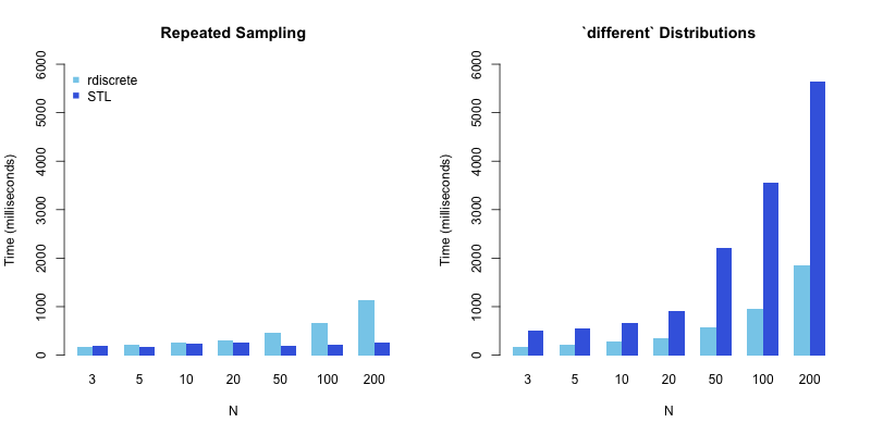
| Figure 1: Sampler timings. The time required for both sampling functions to generate 10 million samples for varying N, the number of possible outcomes. The left-hand panel shows repeated sampling from a single distribution, while the right-hand panel shows repeated sampling from different distributions. |
|---|
Sampling different distributions
The second case of interest is sampling from different distributions. For the STL method, this requires redefining the std::discrete_distribution object for each new sample. Following the same assumption as before, calculating the normalising constant is done once upon object definition; in this case, we assume the normalising constant is not known and use the appropriate version of our function. For our simple function, a new vector of weights is passed to the function for each new sample. The right-hand panel of Figure 1 shows that the STL object becomes much slower when needing to sample from a different distribution, increasing its sampling time rapidly. The hard-coded function also sees an increase in sampling time, but one that is less drastic.
Final remarks
Depending on the use case, and whether you are repeatedly drawing from the same distribution or not, you may want to choose either option. The function(s) provided here are simple and do not require the use of a random number generator object, such as std::default_random_engine, instead depending on the rand function. This is convenient for a compact example, but for serious statistical simulation the random number facilities in <random> are usually preferable because they give greater control over the generator and distribution being used. The functions provided here also have the benefit of not depending on any STL package (with slight modifications to use C-style arrays and remove the std::domain_errors), which may not always be available or desired.