Before discussing Bayesian classifcation methods we intoduce the concept of mixture models, often used for unsupervised classification tasks. Mixture models are a diverse set of statistical models which can take an endless number of forms, the discussion here is limited on finite mixture models. The most common form of which is likely the Guassian mixture model (GMM), used for a variety of applications including clustering, an unsupervised classification method, and traditional modelling. Mixture models are often used to cluster like data-points into groups. In the Bayesian paradigm this is done by inferring a latent classification variable for each data-point.
It is assumed the reader is familiar with the Bayesian paradigm and is compfortable with the notion of statistical modelling. The former is discussed here.
Mixture distributions
A mixture distribution is defined as the weighted sum of multiple probability density functions. Let $f_1(x), f_2(x), \dots, f_k(x)$ be probability density functions, and $w_1, w_2, \dots, w_k$ a set of weights, such that $w_i\geq0$ for all $i$ and $\sum_i w_i = 1$. Then the mixture distribution, $f(x)$, is defined as $$ f(x) = \sum_{i=1}^k w_i f_i(x). $$ Note that if the component densities are well defined, then the mixture density integrates to 1, and all values are non-negative, as required for a probability density function (PDF). The component densities, $f_1(x), f_2(x), \dots, f_k(x)$, should all be appropriately discrete or continuous and have the same dimension for the random variable. However, it is not required that they have the same density with different parameters, and mixtures can combine distributions of various types.
A mixture distribution can be useful when dealing with multimodal or skewed data that is not representative of a standard distribution. In Bayesian statistics, mixture distributions also provide greater flexibility in the choice of prior beliefs.
Normal mixture distribution example
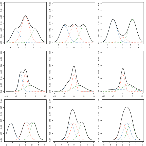
To illustrate the flexibility of mixture distributions, consider a three-component normal mixture distribution. Let $X$ be a random variable described by the mixture distribution, and $\pi_i, \mu_i$ and $\sigma_i$ be the weight, mean and standard deviation of the $i$-th component. The distribution can be written as $$ X \sim \pi_1 \text{N} \left(\mu_1, {\sigma_1}^2 \right) + \pi_2 \text{N} \left(\mu_2, {\sigma_2}^2 \right) + \pi_3 \text{N} \left(\mu_3, {\sigma_3}^2 \right). $$
Figure 1 shows the PDF with a range of parameter values; it is clear from this that a wide variety of densities are possible from just the combination of normal distributions. The endless variety in the density functions available when considering mixture distributions means they are popular prior distributions in Bayesian statistics, when standard distributions are not capable of appropriately capturing prior beliefs.
|
|---|
| Figure 1: Variety of three-component normal mixture distribution. Each row alters only a single parameter. The top row of distributions alters the proportion of the red component, decreasing from left to right and splitting the weights evenly between the other two components. The middle row alters the variance of the blue component, increasing from left to right. The bottom row only changes the mean of the blue component and all other parameters are kept the same. |
Mixture modelling
A mixture model combines appropriately weighted component models to form a single model, representing the natural extension of mixture distributions. The weights associated with each component can be interpreted in two ways: the proportion of the population belonging to the component or the probability that a new observation belongs to that component.
Mixture models can be beneficial when data shows ’like’ sub-populations, groups within the dataset, and exhibit inter-group variation. A major benefit of this model type is that group labels are not needed. In fact, a physical interpretation of the groups is not required, and identification of ’like’ groups can lead to further investigation. Consequently, mixture models can be used to classify datasets into sub-populations, often referred to as clustering. Unlike other clustering algorithms, the number of sub-populations must be chosen before modelling begins. However, this does not stop the fitting of multiple models with varying numbers of components and comparing model fit.
Let ${\boldsymbol{x}, \boldsymbol{y}}$ denote a dataset of $n$ independent observations on explanatory variable $x$ and response variable $y$, such that $\boldsymbol{x} = (x_1, x_2, \dots, x_n)^\text{T}$ and $\boldsymbol{y}=(y_1, y_2, \dots, y_n)^\text{T}$, and suppose that it is believed that the data split naturally into two groups. The first group is modelled by $f_1(y |\theta_1, x)$ and the second by $f_2(y |\theta_2, x)$, with respective weights and model parameters $w_1, w_2, \theta_1$ and $\theta_2$. The mixture model, $f(y|\theta_1, \theta_2, x)$, is defined $$ f(y|\theta_1, \theta_2, x) = w_1 f_1(y|\theta_1, x) + w_2 f_2(y|\theta_2, x). $$ More generally, a $J$-component mixture model is written as $$ f(y|\boldsymbol{\theta}, x) = \sum_{j=1}^J w_j f_j(y|\theta_j, x), $$ where $\boldsymbol{\theta}=(\theta_1, \theta_2, \dots, \theta_J)$, the set of component parameters. The general likelihood function, for observations $\boldsymbol{y}$, is $$ L(\boldsymbol{\theta} | \boldsymbol{x}, \boldsymbol{y}) = \prod_{i=1}^n \left\lbrace \sum_{j=1}^J w_j f_j\left(y_i|\theta_j, x_i\right) \right\rbrace. $$ By expansion of the likelihood, it is clear that this becomes increasingly complex when components or data are added. In particular, the likelihood is an $n$-degree polynomial in the component weights. Therefore, evaluating the likelihood directly is dificult. The calculation can, however, be simplified by the inclusion of the latent variables indicating component belonging for each data-point. Consequently, being inferring the latent states the data is clustered into $J$ groups.
Latent states
Classification by mixture model is the task of learning the unobserved, latent states, which identify each observation as belonging to a model component or sub-population. The latent states are, as such, categorical variables, taking values in the range ${1,2,\dots, J}$, where $J$ is the number of components.
Suppose the group allocation is known, i.e. the data is labelled. The model and likelihood function becomes $$ L\left(\boldsymbol{\theta} | \boldsymbol{x}, \boldsymbol{y}, \boldsymbol{w}, \boldsymbol{Z}\right) = \prod_{i=1}^n w_{Z_i} f_{Z_i} ( y_i | \theta_{Z_i}, x_i). $$ Simplifying the model density removes the $n$-degree polynomial in the likelihood function, drastically decreasing its computational complexity. Evaluation of the likelihood function is critical to many parameter inference schemes in both frequentist and Bayesian settings. As such, including the latent variables could reduce the computational costs associated with inference and facilitate data classification in the process.
Classification and latent state inference
Conditioning the likelihood function on latent states can reduce its complexity. However, latent states are not necessarily known; when this is the case, the latent states must be inferred. In Bayesian methodology, all unknown quantities are treated in the same manner, and so we aim to find the posterior distribution of the latent states.
Let $Z_i$ be the latent state of the $i$-th observation, which is distributed according to the component weights a priori, $$ \text{Pr} \left( Z_i = j | \boldsymbol{w} \right) = w_j. $$
Inference for the latent states can progress by considering their full conditional distributions (FCDs). The law of conditional probability implies that the FCD is proportional to the joint density, $p\left(\boldsymbol{y}, \boldsymbol{Z}, \boldsymbol{\theta}, \boldsymbol{w} \right)$. The probability can be calculated up to proportionality, and so any function not dependent on $Z_i$ can be ignored $$ \begin{aligned} \text{Pr} \left(Z_i = j | \boldsymbol{y}, \boldsymbol{x}, \boldsymbol{\theta}, \boldsymbol{w}\right) &\propto p\left(\boldsymbol{y}, \boldsymbol{Z}, \boldsymbol{\theta}, \boldsymbol{w}\right), \\ &= p\left(\boldsymbol{y}, \boldsymbol{Z} | \boldsymbol{\theta}, \boldsymbol{w} \right) p (\boldsymbol{\theta}, \boldsymbol{w}), \\ &\propto p\left(\boldsymbol{y} | \boldsymbol{Z}, \boldsymbol{\theta}, \boldsymbol{w}\right) p\left(\boldsymbol{Z} | \boldsymbol{\theta}, \boldsymbol{w}\right), \\ &= \prod_{l=1}^n p\left(y_l, | Z_l, \boldsymbol{\theta} \right) p\left(Z_l | \boldsymbol{w}\right), \\ &= p\left(y_i, | Z_i, \boldsymbol{\theta} \right) p\left(Z_i | \boldsymbol{w}\right), \\ &\propto w_j f_j\left( y_i | \theta_j \right). \end{aligned} $$ The joint density, $p(\boldsymbol{y}, \boldsymbol{Z} | \boldsymbol{\theta}, \boldsymbol{w})$, is split into the observed data likelihood, $p(\boldsymbol{y} | \boldsymbol{Z}, \boldsymbol{\theta}, \boldsymbol{w})$ and the latent state density $p(\boldsymbol{Z}|\boldsymbol{\theta}, \boldsymbol{w})$, and simplified. The probability that the $i$-th observation is classified as belonging to the $j$-th component is found to be proportional to the weighted density of the $j$-th component, evaluated at $y_i$. After calculating the normalising constant, the posterior probability can be written exactly, $$ \text{Pr} \left(Z_i = j | \boldsymbol{y}, \boldsymbol{x}, \boldsymbol{\theta}, \boldsymbol{w}\right) = \frac{ w_jf_j\left( y_i | \theta_j \right) } { \sum_{k=1}^J w_k f_k\left( y_i | \theta_k \right)}. $$ This classification naturally arises from the Bayesian mixture model; as such, it is called the Bayes classifier. Inference for other model parameters can proceed using an appropriate inference scheme by conditioning on latent states. At each iteration of the inference scheme, the latent states for each observation are then randomly assigned using the above probability mass function.
# Label switching
Label switching is an issue seen during the inference of mixture model parameters. Consider the two-component mixture model, $$ f(y | \theta_1, \theta_2, \pi, X) = \pi f_1(y|\theta_1, x) + (1-\pi)f_2(y|\theta_2, x), $$ where $f_1$ and $f_2$ are the same model family, i.e. both normal distributions. The problem arises due to the exchangeability of parameters, that is, the model, $f(y | \theta_1, \theta_2, \pi, x)$ is indistinguishable from $f(y | \theta_2, \theta_1, 1-\pi, x)$. The result of this exchangeability is that the Markov chains targeting the posterior $p(\theta_1 | \boldsymbol{y})$ and $p(\theta_2|\boldsymbol{y})$ can jump between the two states. This can lead to errors when inspecting posterior moments of the distributions and errors when inspecting predictions drawn from the model. If label switching has occurred, it is often evident from inspecting trace plots and convergence diagnostics. Autocorrelation would appear to be extremely high, and the chains will have a large within-chain variation leading to a high $\hat{\text{R}}$.
Theoretically, it is possible to prevent label switching through a careful selection of prior beliefs; however, this is not guaranteed to work, and such beliefs may not accurately represent the true beliefs. A more practical approach is to impose a constraint on the parameters $\theta_1$ and $\theta_2$. Enforcing $\theta_1<\theta_2$ within the inference scheme can prevent the two chains from jumping between the posterior distributions. The ordering constraint does impose some restrictions on posterior analysis. Suppose we wish to know the probability that $\theta_1>\theta_2$. In the Bayesian paradigm, the probability is approximated by the proportion of posterior draws such that $\theta_1>\theta_2$, which will be zero due to the imposed constraint. Additionally, imposing this constraint becomes more difficult when the number of unknown parameters is high.
Another approach is to initialise the Markov chain at realistic initial values, close to the posterior modes. Again, this does not guarantee that the chains will not transition between modes, and selecting appropriate initial values may prove challenging.
Final remarks
In this post we introduced mixture modelling and how these models can be used for unsupervised classification of data-points within the Bayesian paradigm. Consequently, mixture distributions were also introduced, hopefully their versatily was demonstrated in generating non-standard distributions, which is particularly useful in Bayesian analysis.