The t-test is one of the most common tests used in statistics. It compares the means of two normally distributed datasets by calculating a test statistic and comparing it to the t-distribution. Variations of the test exist, including constant and differing variance between groups, paired and unpaired, and non-normality in the data. Here, Bayesian hypothesis testing is discussed, giving an indication of how a two-sample t-test would be conducted within a Bayesian context. Extensions to other situations are available, but the focus of this is to illustrate the how hyptothesis testing is done within the Bayesian paraidgm.

Also introduced are high-density intervals (HDIs), which are a key aspect of Bayesian hypothesis testing. HDIs these are akin to confidence intervals (CIs) commonly used within frequetist methods. It is assumed that the reader has some familarity with Bayesian methods, if not this post should introduce all necessary prerequisits.

Hypothesis testing

Let \(\left\lbrace \boldsymbol{X}_{1}, \boldsymbol{X}_{2} \right\rbrace\) be two independent and normally distributed datasets, with means \(\mu_{1}\) and \(\mu_{2}\). Assume the variance of the two groups are known and equal, although this need not be the case. In a Bayesian context, the posterior distributions \(p(\mu_{1}|\boldsymbol{X}_{1})\) and \(p(\mu_{2}|\boldsymbol{X}_{2})\) are inferred, in the usual manner by constructing a prior distribution and combining with the data likelihood. Let the difference of the group means define a random variable, \(\Delta \mu = \mu_{1} - \mu_{2}\). The posterior distribution \(p(\Delta\mu | \boldsymbol{X})\) where \(\boldsymbol{X} = \left\lbrace \boldsymbol{X}_{1}, \boldsymbol{X}_{2} \right\rbrace\), is of interest here and can be found either analytically or by MCMC, by either method, the difference in the group means can be inspected by analysing \(p(\Delta\mu | \boldsymbol{X})\). For example, to answer the question; Is the mean of group 1 larger than group 2? A Bayesian statistician would calculate the posterior probability \(\text{Pr}(\mu_{1}>\mu_{2}| \boldsymbol{X})\), which is equivalent to \(\text{Pr}(\Delta\mu>0|\boldsymbol{X})\). If \(p(\Delta\mu | \boldsymbol{X})\) is found via MCMC, the probability is approximated

\[ \text{Pr}\left( \Delta\mu > 0 | \boldsymbol{X} \right) \approx \frac{1}{N_{\text{MCMC}}}\sum_i \mathbb{I}(\mu_{1}^{(i)} > \mu_{2}^{(i)}) \]

where \(N_{\text{MCMC}}\) is the number of posterior realisations and \(\mu_{1}^{(i)}\) and \(\mu_{2}^{(i)}\) are the \(i\)-th realisations from the posterion. the indicator function, \(\mathbb{I}(\cdot)\), equals 1 if the expression is true and zero otherwise. Although a Bayesian statistician would not use the word significant, they may say that if the probability is low, less than 0.05, then there is substantial evidence to suggest that the mean of group 1 is larger than the mean of group 2.

Other questions regarding the two group means can be proposed, and their answer formulated in a similar manner by inspection of the appropriate posterior distribution.

An important aspect of hypothesis testing in frequentist statistics is the confidence interval. In the Bayesian context, an analogue of the confidence interval is often used, the HDI. Their uses are very similar to the confidence interval (CI), but their theory is based on the parameter beliefs rather than asymptotic assumptions via the central limit theorem. Here, HDIs and introduced and how they differ from a CI is discussed.

High density intervals

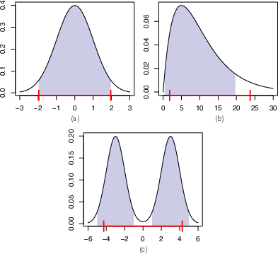
For a univariate random variable, a $100(1-\alpha)$% HDI defines a region of the support such that; for all points within that region, the density function is larger than for all points outside that region and intergal over that region evaluates $(1-\alpha)$. The former condition ensures that the region is unique, assuming that the density is not flat at any point within the interval. While the latter ensoure that the region is of the correct size.

For example, consider the distribution in Figure 1. The symmetric distribution in Figure 1(a) has the same HDI as an equi-tailed confidence interval. When the distribution is skewed or bimodal, such as Figures 1(b) and 1(c), this is not the case. The equi-tailed confidence interval for a skewed distribution is shifted compared to the HDI. The HDI of the bimodal distribution in Figure 1(c) contains the two modes but does not contain the mean, zero. For bimodal and skewed distributions, the use of CI does not make sense, and HDIs are preferred, but for symmetric distributions there is little difference.

Figure 2: High density intervals compared to equi-tailed confidence intervals. High-density intervals for (a) unimodal, (b) skewed, and (c) bimodal distributions are illustrated by the shaded blue area below the density curve. Equivalent equi-tailed confidence intervals are shown by red bars along the $x$-axis.

In statistics, it is often of interest whether a quantity is significantly different from zero. To answer this, often the 95% CI for that quantity is compared to zero, and if zero lay outside of that interval there is evidence to suggest that the quantity is significantly different from zero. In Bayesian context, we check that zero lie outside of the HDI and, if so, we say there is substantial evidence that quantity is not zero.