Introduction

Electricity differs from many financial and commodity assets because large-scale storage remains expensive, requiring supply and demand to be balanced continuously. In the UK day-ahead market, hourly electricity prices are determined through auctions that incorporate expected generation, demand, and transmission constraints. In Great Britain, this balance is overseen by the National Energy System Operator (NESO), which manages the grid through a combination of forward markets and a real-time Balancing Mechanism. A key feature of the UK energy market is the day-ahead auction, which is facilitated by two exchanges: EPEX SPOT and Nord Pool’s N2EX. The auctions operate such that all successful buyers and sellers receive the same clearing price, despite the large difference in cost to produce electricity between renewable and non-renewable methods. The price is determined by the most expensive energy producer to be accepted for that period; this is called the marginal price. The spot prices today were, therefore, set in yesterday’s auctions. Both producers and suppliers commit to their positions a day ahead.

Accurately forecasting the energy spot price is, therefore, of interest to both energy producers and users. Producers could increase supply if energy prices rise to a sufficient amount, or equally reduce supply when the spot price is too low. Similarly, large-scale energy users could shift intense energy usage to periods of lower prices. In recent years, forecasting energy spot prices has grown considerably more challenging, as the UK’s renewable energy production has increased drastically. The weather-dependent nature of renewable production means that energy production can drop or spike unexpectedly, causing a spike in spot prices. Unexpectedly high renewable output can cause prices to drop, and even go negative; similarly, unexpected drops in renewable output can cause prices to spike as more expensive gas and coal are required to cover the shortfall.

This blog continues the investigation of modelling energy spot prices within Great Britain from my other blog post. The aim of this blog is the same as the other, to build and compare models of energy spot prices within Great Britain. Here, however, the focus is on stochastic models, whereas previously we used statistical models of time-series data. Energy spot prices exhibit complex dynamics which classical statistical models may fail to capture, such as mean reversion, price spikes and volatility clustering; these features make stochastic models an excellent tool for forecasting spot-price dynamics. Such models are essential for pricing forward contracts and derivatives in the energy market, where accurately predicting expected price and uncertainty is key for valuation and risk management.

The data

The data is sourced from Transmission System Operators and power exchanges, and is available through kaggle. A detailed description of collection methods and data structure is given on a GitHub page. The dataset is large, containing observed spot prices in many regions and a range of explanatory variables. Here, we restrict the dataset to hourly energy spot-prices determined on the day-ahead auction. The data, however, contains some missing values, which are filled using a smoothed Kalman filter when modelling begins, to avoid added difficulties of missingness during parameter inference.

The dataset spans the years 2014 to 2020, resulting in thousands of hourly observations, as seen in Figure 1. The spot price appears to remain close to an overall mean with large sporadic deviations away from this, before returning to its base state. These deviations are referred to as spikes and are important when considering modelling the data. In this blog, stochastic models of energy price data are fit and compared by their predictive power and model performance.

Methods

We propose, fit, and compare several stochastic models of energy spot price. For this, the dataset is split into training and validation subsets, where the final month of data is reserved for model validation. Due to the computational cost of parameter inference, the training dataset is a subset of the original dataset and contains two years (assumed to be 730 days) worth of data, starting from 02/09/2018.

Models are compared based on their model fit to the training data and their predictive performance for the validation dataset. The focus, however, is on the within-sample model fit, which investigates which model can most accurately represent the dynamics of energy spot price. Parameters are inferred within the Bayesian paradigm, which is well suited to handle models with hierarchical and complex structures. Inference is done within Stan, a probabilistic programming language which implements a Hamiltonian Monte Carlo (HMC) no-U-turn algorithm to efficiently sample from the targeted joint posterior distribution. All scripts related to this work can be found in the GitHub repository.

All models combine a deterministic mean function and stochastic component. The mean function does not differ between models; however, its parameters are inferred with the stochastic component’s as one inference scheme, and so they can differ between models. We chose to model the spot prices directly (not on the log scale), allowing negative prices, a known spot-price phenomenon caused by periods of excess generation, often caused by high renewable output and an inability to shut down non-renewable generators due to operational constraints. Let $S_t$ denote the spot price at time $t$; the general form of the models is

where $\Lambda_t$ is the deterministic mean function, evaluated at $t$, and $X_t$ is the stochastic component. The form of the deterministic mean function is discussed first, and the stochastic components are introduced after.

Mean function

The data show seasonal trends in the spot price as a result of predictable changes in energy’s supply and demand. This trend should be incorporated into a model to improve predictive performance and not rely purely on the stochastic variation to predict spot price. The proposed mean function combines categorical indicators for day of the week and hour of the day, and a yearly trend modelled by a linear trend and a third order fourier series to capture the yearly variation. That is,

where $\mu_0$ is an overall mean and $\mu_1$ is the linear time trend. The variables $A_t$ and $B_t$ indicate the weekday and hour, respectively, and, therefore, $\beta_i$ and $\gamma_i$ are the daily and hourly effects on spot price. Lastly, the yearly trend in the data is captured by the Fourier series (and linear trend); the order of the series is limited to three to not over-fit to the training data.

Mean-Reverting Process

A mean-reverting stochastic process drifts towards a defined long-term mean, unlike a pure Brownian motion process whose value is entirely random; the process has a bounded variance in the time limit. In the energy market, mean-reversion is driven by a number of factors, including supply-demand balancing, weather normalisation and the balancing market. Mathematically, mean-reversion is achieved by incorporating a drift proportional to the negative of the process’s current value, i.e. inducing a positive movement if the current value is below the long-term mean and vice versa; the speed of reversion is controlled by a parameter, $\theta$. The process also includes a volatility parameter, $\sigma$. Here, we assume the long-term mean is zero, as the deterministic mean function, $\Lambda_t$, is intended to model the expected seasonality in spot price. The stochastic differential equation (SDE) defining the process is

The transition density for a mean-reverting process can be found in closed form, allowing the spot-price transition density to also be written in closed form. where $\Delta t$ is the time-step between observations. Modelling the spot price in hourly time units and having hourly data observations implies that $\Delta t=1$ and it is dropped from future equations. The closed form of the transition density allows the model likelihood to be calculated without approximation of the process, allowing for inference to proceed relatively easily. The closed form solution also allows exact forward-simulation of the sample path.

Inference

Bayesian inference requires the specification of prior beliefs. Where appropriate, the estimates from the training dataset are used as expected value a prior; this is for the volatility and overall mean of the deterministic function. In these cases, the priors can show fairly high degrees of certainty in their value; elsewhere, relatively weak prior beliefs are used. The inference, implemented via Stan, is relatively fast, taking under 10 mins to execute four independent chains with 1,500 iterations, of which the first 500 are removed for burn-in. Inference was executed using a 2024 MacBook Pro with an M2 chip and 16Gb RAM. However, it is noted that extracting posterior predictives using Stan incurs a much larger computational burden, exhausting available RAM, and so these are done in Python post inference. Writing posterior sampling code outside of Stan means that computational efficiencies such as vectorisation, and where appropriate, parallel sampling can be utilised. Importantly for this case, it also allows direct control over which variables are stored and returned, to not exhaust available RAM. For all models discussed here, posterior sampling is done directly in Python, and the Stan scripts only return posterior draws.

The posterior chains are checked for convergence to the same posterior distribution by the R-hat statistics, which measure inter- and within-chain variability. The generally accepted rule is that a value of less than 1.05 implies that there are no signs that the chains have not converged. The R-hat value is calculated separately for each parameter in the model, and all values are below the accepted threshold. We also inspect the effective sample size (ESS), which estimates the equivalent number of truly uncorrelated posterior draws which the chains have produced. A high ESS indicates that the chains have little autocorrelation. Again, the ESS is calculated individually for each parameter. Here, the minimum value is around 1,000, and the parameters with the lowest ESSs are the overall mean and hourly effects of the mean function, suggesting high posterior autocorrelation. Further inspection shows the hourly effects posteriors are highly correlated with neighbouring hourly effects, possibly explaining the high autocorrelation.

Posterior Predictions

The resulting posterior predictive plots can be seen in Figure 1. The model appears to capture the shape of the training data fairly well. An example posterior one-step-ahead predictive density is also shown. We see that it fails to capture the fat tails synonymous with energy spot price. The validation dataset lies mostly within the predictive density, although it seems to have a higher overall mean level than the model predicted. This may be due to a general rise in spot price which the model hasn’t accounted for, seen in increasing spot price in the final few months of the training data. Lastly, a sample path drawn from the stochastic process a posteriori does not reflect the spikes seen in the data and appears to have an overall higher volatility than the spot price in its usual state. This is likely due to inadequacies of the model being unable to replicate spike behaviour.

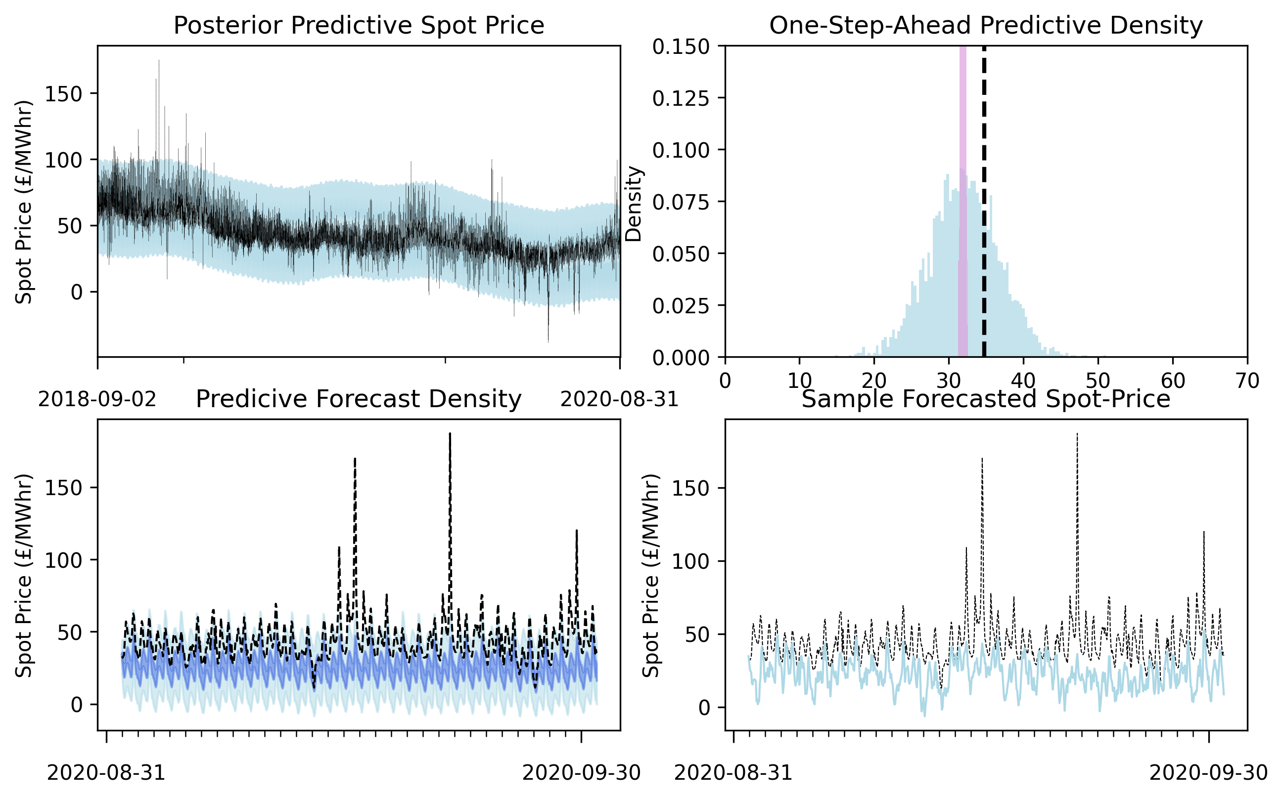
Figure 1: Mean-Reverting Process’s Posterior Predictives. (Top left): Training data (black line) and 99% posterior predictive interval (light blue shaded region). (Top right): Posterior one-step-ahead predictive density of the final observed dataset (light blue histogram) and the one-step-ahead posterior expected value (pink histogram) plotted against the observed final value (dashed black line). (Bottom left): Posterior predictive forecast and validation data. The 99% posterior predictive interval is shown by the blue shaded region and middle 50% predictive region is shaded dark blue. (Bottom right): The validation dataset and a sample path of the process a posteriori.

Mean-Reverting Jump Process

Although mean-reversion captures the overall trend of the data, it is not capable of reproducing the large tails in spot-price distribution from Brownian stochasticity alone. Hence, we wish to introduce larger spikes and increased volatility into the process. This can be done by the inclusion of discontinuous jumps. Large jumps in spot price are a known phenomenon and can be seen clearly in this dataset. They can be caused by a range of issues such as power plant outages, errors in renewable generation forecasting, and changes in the price of gas. The SDE below describes a mean-reverting process with an additional component, denoted $J_t\text{d}N_t$. Where $J_t$ is a discontinuous jump at time $t$, and $N_t$ describes a Poisson process with constant rate $\lambda$. The Poisson process allows jumps in energy price to arrive randomly, reflecting large price spikes. The jump-size parameter is itself a random variable described by a distribution. Price spikes both increase and decrease the spot price and, hence, its range should be the whole real line. Reflecting this, jump sizes are assumed to be normally distributed, and the stochastic component of the model is

We assume that the time-step, $\Delta t = 1$hr, is small enough that at most one jump can occur within it. This assumption allows the transition density to be tractable, without the need for considering an infinite number of jumps or approximation. The transition density can then be written as a mixture distribution with weights given by the probability of a jump occurring, $p$, The likelihood is, therefore, also tractable and inference can proceed.

Inference

The model parameters largely overlap with those of the previous mean-reverting model, and where this is the case, the same priors were used. The jump-size parameter, $J_t$, is expected to be centred near zero, as a positive or negative value would skew jumps to be in that direction. Therefore, $\text{E}[\mu_J] = 0$ and $\text{SD}(\mu_J)= 0.1$ are imposed. The jump-size variance is assumed to be large, reflecting the large variety of jump sizes seen in the data and we set $\text{E}[\sigma_v] = 50$ and $\text{SD}(\sigma_v) = 5$, the expected value is intended to be large enough that the variation in the data caused by the jump process is not muddled with that caused by the mean-reverting process, while the prior variance still allows movement away from the prior mean. By convention, a prior distribution is placed on the probability of a jump occurring over the time-step, not the Poisson process rate. This is to avoid numerical instability when exploring very small parameter values, although here the two are equivalent. Jumps are assumed to be rare, and a $\text{Beta}(1,50)$ distribution is used to summarise our prior beliefs.

The inference was executed for four independent chains, all of length 1,500, where the first 500 were removed for burn-in. Inspecting the posterior output, we find that the posterior chains showed no signs of non-convergence, all parameters having an R-hat value below 1.05 and the minimum ESS was approximately 1,400. Similarly to before, the parameters which showed the highest posterior autocorrelation were the hourly effects in the mean function.

Posterior Predictives

The posterior predictives show wider 99% predictive intervals when compared to the previous models. Significantly, the example one-step-ahead predictive density shows fat tails, as a result of the jump process. Similarly to before, the posterior expectation of the validation data lies below the observations; however, the fat tails in its prediction mean the observed data fit more comfortably within the 99% predictive interval. The sample path, however, still does not resemble spikes in energy price. This is likely due to the model’s inflexibility; it assumes the same mean-reversion is used when the spot price is in its usual state and after a spike has occurred. However, the data shows rapid return to the usual spot price; a single reversion rate would not be able to capture both dynamics.

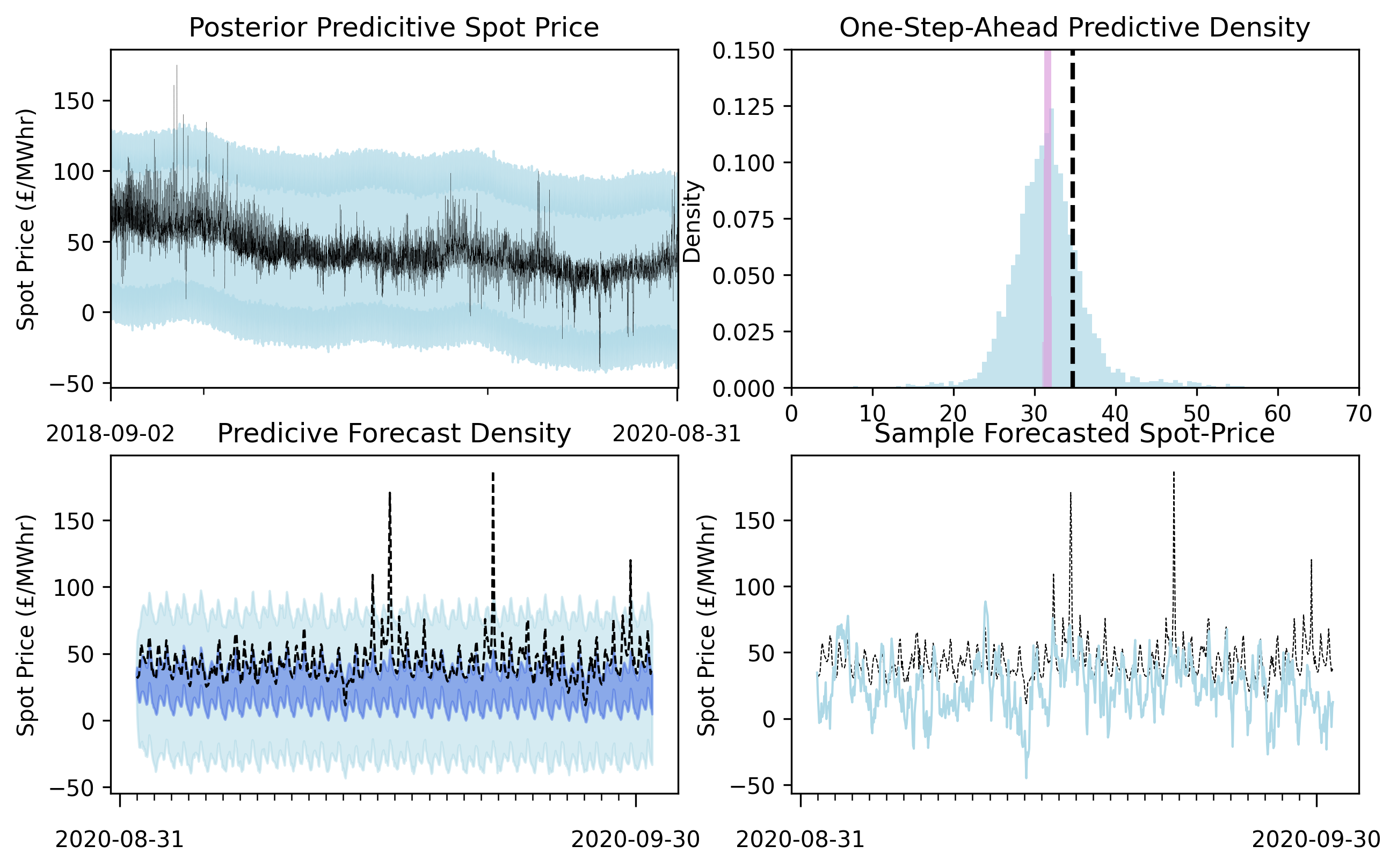
Figure 2: Mean-Reverting and Jump Process’s Posterior Predictives. (Top left): Training data (black line) and 99% posterior predictive interval (light blue shaded region). (Top right): Posterior one-step-ahead predictive density of the final oberserved dataset (light blue histogram) and the one-step-ahead posterior expected value (pink histogram) plotted against the observed final value (dashed black line). (Bottom left): Posterior predictive forecast and validation data. The 99% posterior predictive interval is shown by the blue shaded region and middle 50% predictive region is shaded dark blue. (Bottom right): The validation dataset and a sample path of the process a posteriori.

Regime-Switching Diffusion Model

Another modelling approach is to assume that the energy price is governed differently depending on whether the price is currently within a spike or whether it is in its usual (non-spike) range, referred to as a ‘base regime’. This distinction can be incorporated into a model by introducing a latent variable indicating the underlying state: base or spike. The base regime, $X^b_t$, is modelled using a mean-reverting component with discontinuous jumps following a Poisson process, while the spike regime, $X^s_t$, follows an independent mean-reverting process, with different parameters;

The latent process, the unobserved regime, can be considered to be a Markov chain, whose current state, $Z_t$, depends only on the previous, $Z_{t-1}$. The chain is described by a transition matrix, whose probabilities are to be inferred. This type of model is also called a hidden Markov model and also falls into the category of state space models. The latent process adds some complexity to calculating the likelihood, where all paths of the underlying state space must be considered. However, this calculation can be simplified by using the forward algorithm. It iteratively calculates the probability of the current and the next state given the data up until that point. By using this algorithm, the likelihood can be calculated, and inference can proceed.

Inference

The prior beliefs for the base regime follow those from the previous model. The reversion rate and volatility of the spike regime are assumed to be higher than those of the base regime, reflecting a quick return to the usual spot-price range after a spike, and priors were constructed to reflect this. However, regime-switching models can suffer from label switching. To overcome this, it is assumed that the spike regime has a larger reversion rate and volatility, and we constrain $\theta_b<\theta_s$ and $\sigma_b<\sigma_s$.

We must also construct prior beliefs for the transition matrix and initial state. Given the low occurrence of spikes, we have firm prior beliefs that the first observation comes from the base regime, and so a Dirichlet distribution is employed to reflect this. The transition of the latent states of the process must also be given a prior distribution. The model intends for the spot price to vary under the base regime in usual conditions and the spike regime to model a return to those conditions; therefore, we assume a large weight that, if in the base regime, the latent state stays there and if in the spike regime, the Markov chain moves to the base regime. A Dirichlet prior is used for the rows of the transition matrix to reflect this.

The complexity of the model reflected the complexity of posterior probability space, and the inference scheme struggled to converge to a single posterior distribution. To prevent this, the probability of a jump occurring over a time-step was fixed at the posterior mean of the jump probability when fitting the previous model. The interpretation of the two parameters is the same, and the addition of a second regime here is intended to model the return to the base regime and should not affect the jump probability. The posterior chains showed no signs of non-convergence, all with R-hat values within an acceptable range. The parameters with the lowest ESSs were the hourly effects in the mean function, which showed high posterior correlation with their neighbouring hour effects, yet these all still have an ESS above 1,000.

Posterior Predictives

The example one-step-ahead predictive density shows some indication of fat tails, caused by spikes, but they are less prominent than in the previous model, see Figure 3. The posterior sample path shows some spikes, although their magnitude is lower than what is observed in the data. The posterior predictive intervals reflect those of the previous model.

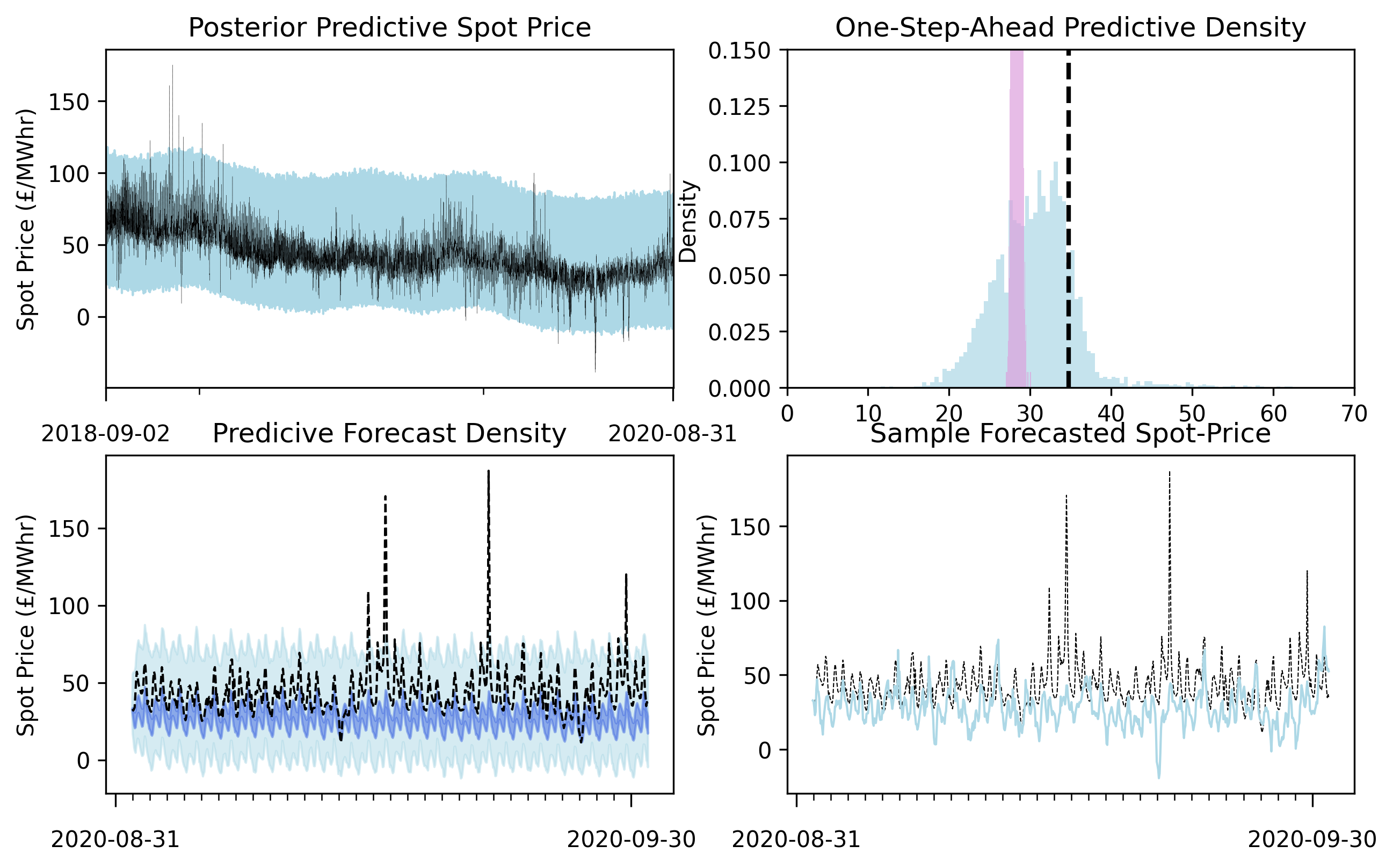
Figure 3: Markov Regime Switching Model’s Posterior Predictives. (Top left): Training data (black line) and 99% posterior predictive interval (light blue shaded region). (Top right): Posterior one-step-ahead predictive density of the final oberserved dataset (light blue histogram) and the one-step-ahead posterior expected value (pink histogram) plotted against the observed final value (dashed black line). (Bottom left): Posterior predictive forecast and validation data. The 99% posterior predictive interval is shown by the blue shaded region and middle 50% predictive region is shaded dark blue. (Bottom right): The validation dataset and a sample path of the process a posteriori.

Stochastic Volatility

The final model considered in this blog is a model which includes dynamic, time-varying volatility. The models so far have considered the volatility to be constant, although the regime-switching model allows the volatility to vary between regimes. Here, we propose a model where the volatility is considered stochastic and an unobserved latent process within the system. The log-volatility, $V_t$, is modelled by a mean-reverting process with discontinuous jumps described by a Poisson process with constant rate. The jumps in log-volatility are intended to propagate and increase volatility in the stochastic process $X_t$, allowing for large-tailed predictive distributions for the spot price. The model is,

where $\sigma_t = e^{V_t}$ and the Browian motion processes, $\text{d}W_t^V$ and $\text{d}W_t^X$, are assumed to be independent. The jumps in log-volatility are, similarly to before, assumed to be normally distributed with mean and variance to be inferred, allowing jumps in both directions and letting the transition densities be tractable.

Inference

The complexity of the model means that it is hard to distinguish between variation in spot-price caused by variation in spot-price stochasticity or the log-volatility dynamics. To aid inference, setting some parameters to realistic values can allow inference to proceed with the remaining parameters. The jump in log-volatility is intended to reflect the increased volatility which leads to a spike in the spot-price. The rate of this was previously inferred in the mean-reverting jump-process model. Therefore, we fix the probability of the jump in log-volatility, over the time-step $[t, t+\Delta t)$, to be the posterior mean of the probability of a jump in spot-price inferred from the earlier model. This parameter fixing allows inference to proceed for the remaining parameters.

Prior beliefs for the log-volatility process are hard to construct as it is completely unobserved. The logged rolling standard deviation of spot-price is inspected to gain some idea of value of the parameters which govern model and the prior expectations $\mu_v$ and $\sigma_v$ are set the mean and standard deviation of the logged rolling standard deviation of the observed spot-price. The prior uncertainity is, therefore, considered low and set $SD(\mu_v)=0.1$ and $SD(\sigma_v)=0.1$. The remaining overlap with previous and the same priors are used.

The model complexity results in a higher computational burden, and four chains with 1,500 iterations requiring over two hours to be inferred in Stan. The time required is, however, not the restricting factor and Stan exhausts the RAM of a 16Gb machine when attempting to compile and return the posterior draws. Therefore, chains were executed with 1,000 iterations, the first 500 being removed for burn-in. Further, one of the chains showed clear signs of non-convergence and was removed from the posterior draws, once removed the R-hat statistics for all parameters where within the acceptable range of convergence (<1.05). The ESS for the parameters ranged from 244 to 2,930, with the parameters $\mu_v$ and $\theta_v$ having the lowest ESSs.

Posterior Predictions

The posterior predictives of this model resemble those seen in others; however, the example one-step-ahead predictive density clearly shows fat tails reflecting the spot-price phenomenon. The posterior sample path is also the only path to clearly show a distinct spike in spot price akin to those in the data. The posterior expected values for the validation dataset are still below the observed data, reinforcing that this is an issue with the mean function data capturing the increase in spot price.

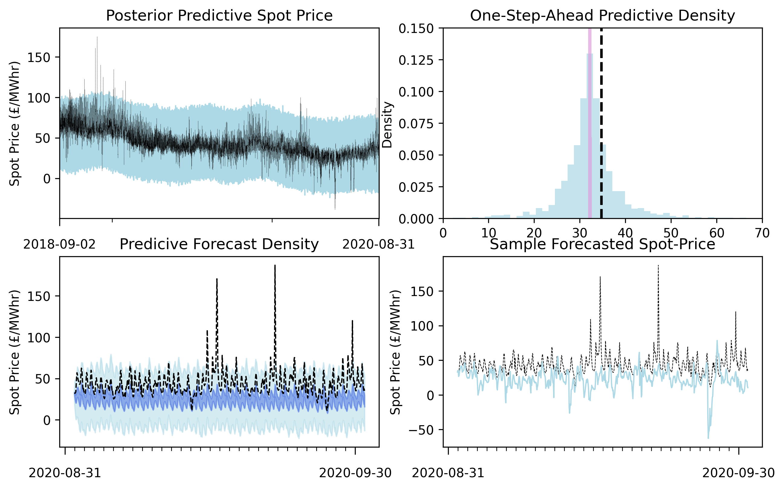
Figure 4: Stochastic Volatility Model’s Posterior Predictives. (Top left): Training data (black line) and 99% posterior predictive interval (light blue shaded region). (Top right): Posterior one-step-ahead predictive density of the final oberserved dataset (light blue histogram) and the one-step-ahead posterior expected value (pink histogram) plotted against the observed final value (dashed black line). (Bottom left): Posterior predictive forecast and validation data. The 99% posterior predictive interval is shown by the blue shaded region and middle 50% predictive region is shaded dark blue. (Bottom right): The validation dataset and a sample path of the process a posteriori.

Results

Mean function

Here, only a single mean function was considered, which may not be the most appropriate. Although a common form of mean function used within spot-price modelling, it may not be the best fit for this particular dataset. The function captures the trend of the data; however, upon inspection, the deseasonalised spot price diverges from zero, particularly in the first and last months of the training dataset see Figure 5. This explains the higher-than-observed spot price in the validation dataset across the models.

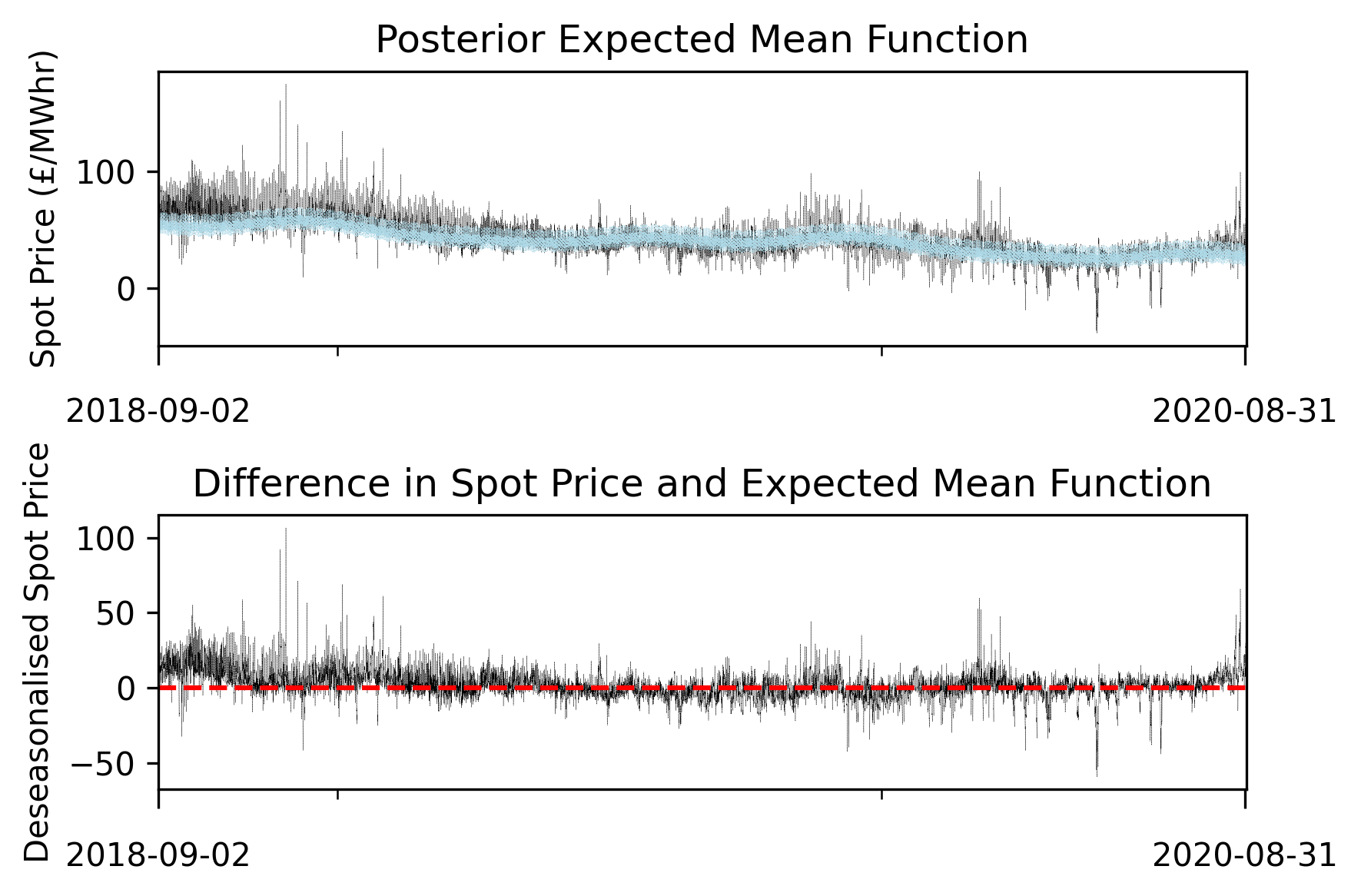
Figure 5: Posterior Mean Function and Deseasonalised Data. (Top): Posterior expectated determiniistic mean function (blue) and the training dataset (black). (Bottom): The deseasonalised data, after subtracting the expeected value of the mean function at each point (black) and a horizontal red dashed line at zero.

Stochastic model fit

The models are compared based on both their fit to the observed training data and their predictive performance on the unobserved validation dataset. To directly compare how each model fits to the training data, the expected posterior log-likelihood, and its standard deviation, is reported in Table 1. The model with the largest expected log-likelihood is Markov regime switching model, indicating it shows the best within-sample fit to the data.The Wanatabe-Akaike information criteria (WAIC) is also reported, this is a summary statistics often used in Bayesian statistics that is intended to estimate the models ability to predict unobserved data. The models which have the lowest, and preferred, WAIC are the mean-reverting jump process model and Markov regime switching model, in fact they equal to three significant figures. The stochastic volatility model has the largest WAIC statistic, indicating that it may have the lowest predictive power of the models tested. The final comparison statistic considered is the Log-Score (LS) which is the posterior log-likelihood of the validation dataset. This statistic heavily penalises observations in areas of low posterior density i.e. those which have a very low probability of being observed. Interestingly, the model with highest, and preferred, Log-Socre is the stochastic volatility model. This is contradictory to the WAIC statistics which suggested that the stochastic volatility model was the worst. The apparent difference in their conclusions is due to their calculation. The WAIC statistic averages the expected posterior density, therefore penalising models with low predictive density. However, the fat tails of the stochastic volatility predictive, reduces the density for the remaining (non-spike) spot-prices, increasing its WAIC statistic. In contrast, the LS penalises models with poor performance in the extremes, and thus would “reward” the stochastic volatility models fat tails, where the spiked spot-price have higher posterior denisty. The statistics are, therefore, concerned with different predictive attributes of modelling, and this is reflected in their apparently contradicting results.

Model	MR	MR-JP	MRS	SV
$\text{E}[p(\boldsymbol{y})]$	7.04	7.18	7.21	7.16
$SD(p(\boldsymbol{y}))$	0.00347	0.00442	0.00396	0.0133
WAIC	5.016	5.00	5.00	7.87
LS	-6.90	-4.53	-5.10	-4.77
range LS	(-349, -2.47)	(-43.0 -2.21)	(-40.8, -2.60)	(-13.8, -2.15)

Table 1: Model Fit Summary Statistics.

Limitations

The validation data consisted of the final month of data in the whole dataset. This is relatively small, and although shorter time-scales are also useful, spot-price forecasts are often made several months or years in advance. This was primarily done to reduce the computational burden, which was already significant for the more complex models considered. The computational burden also hindered the prediction types that were made. Time-series data commonly uses a sliding window prediction; however, the cost of this would have been too great for the stochastic volatility and Markov regime-switching models. The computational cost also affected the results of the final model, which had significantly fewer posterior draws than the other models. Added to this was the low ESS of some of its parameters, which may lead to improper summary of their posterior distributions and reduced accuracy in the posterior predictives.

The mean function used here was not able to fully deseasonalise the data, and it was the only one considered. This resulted in the stochastic components modelling spot price data with higher levels of stochasticity than intended; recall the deterministic mean function was meant to account for the expected seasonal variation within the data. Although inspection of the deseasonalised data, it is not obvious which level of seasonality is missing. The Fourier component of the mean is specifically limited to three components to prevent over-fitting to the training dataset; however, this may be too few.

Future work

The models should be tested using a larger validation training dataset and a sliding window prediction. This would require considerable computational cost if the inference continued to be executed in Stan. This, however, may not be the case. By using Sequential Monte Carlo (SMC) methods, the parameter value beliefs could be updated with each window and predictions made without having to re-infer parameters from scratch. SMC essentially treats the current posterior distribution as the prior and updates with the likelihood from the new validation data. This may reduce the cost of inference, but proper calibration and testing of the scheme would be needed and is likely not trivial.

A significant improvement to the models could be made via the mean functions. As mentioned, the proposed function is not able to fully deseasonalise the data, and the stochastic component therefore has to account for additional variation in the data. This should drastically improve model predictions and reduce predictive errors. Here, two variables were included in the mean function; however, other variables which are correlated to energy spot price, such as predicted renewable generation, could make significant improvements to the mean function and model performance. Here, the model of stochastic volatility was shown to be the most capable of capturing the predictive uncertainty of price spikes. The volatility model was relatively simple, and a comparison of other volatility models, such as the Heston model, should be undertaken.

Conclusion

This blog investigates four stochastic models to predict energy spot-price within the UK, under a Bayesian framework. The model which showed the greatest predictive power incorporated stochastic volatility allowing the predictive distributions to have fat tails, commonly seen in spot-price data resulting from price spikes. The inclusion of stochastic volatility in the model, therefore, appears to be an important tool in spot-price modelling. A dynamic volatility allows for periods of high variation, a phenomenon called volatility clustering, which is also known to occur in energy spot prices. The stochastic volatility model used here, although simple, was able to mimic such periods and generate more accurate predictions which could better handle extreme spot-prices seen within price spikes of a validation dataset.

Forecasting spot prices is not only important for energy producers or users wishing to benefit from high demand or low prices, respectively, but also for traders. In recent years, futures contracts on energy spot prices have become more common due to the deregulation of the energy market. Contracts must be priced to avoid risk-free money-making scenarios, known as arbitrage; this involves modelling the price of the commodity and pricing the contract accordingly. Stochastic models have been ubiquitous in such work, as their inherent stochasticity reflects the erratic movement of markets. In practise, traded forward prices are observed from the market and used to calibrate models under a risk-neutral framework. Spot-price models are particularly useful when stress testing portfolios and modelling assets exposed to price volatility, such as energy storage and flexible generation.