Introduction
Electricity differs from many financial and commodity assets because large-scale storage remains expensive, requiring supply and demand to be balanced continuously. In the UK day-ahead market, hourly electricity prices are determined through auctions that incorporate expected generation, demand, and transmission constraints. In Great Britain, this balance is overseen by the National Energy System Operator (NESO), which manages the grid through a combination of forward markets and a real-time Balancing Mechanism. A key feature of the UK energy market is the day-ahead auction, which is facilitated by two exchanges: EPEX SPOT and Nord Pool’s N2EX. The auctions operate such that all successful buyers and sellers receive the same clearing price, despite the large difference in cost to produce electricity between renewable and non-renewable methods. The price is determined by the most expensive energy producer to be accepted for that period; this is called the marginal price. The spot prices today were, therefore, set in yesterday’s auctions. Both producers and suppliers commit to their positions a day ahead.
Accurately forecasting the energy spot price is, therefore, of interest to both energy producers and users. Producers could increase supply if energy prices rise to a sufficient amount, or equally reduce supply when the spot price is too low. Similarly, large-scale energy users could shift intense energy usage to periods of lower prices. In recent years, forecasting energy spot prices has grown considerably more challenging, as the UK’s renewable energy production has increased drastically. The weather-dependent nature of renewable production means that energy production can drop or spike unexpectedly, causing a spike in spot-price. Unexpectedly high renewable output can cause prices to drop, and even go negative; similarly, unexpected drops in renewable output can cause prices to spike as more expensive gas and coal are required to cover the shortfall.
In this post, we investigate a range of time-series modelling techniques to be able to predict the energy spot-price and compare them based on their predictive performance.
The Data
Data source
The data is sourced from Transmission System Operators and power exchanges, and is available through kaggle. A detailed description of collection methods and data structure is given on a related GitHub page. The dataset is large and contains spot prices and explanatory variables for many regions within Europe. The modelling here is limited to data within Great Britain, and the explanatory variables are reduced to those believed to be most important: solar generation, wind generation, and forecasted energy use.
Features of the data
Upon inspection of the data, there appears to be little overall trend in energy spot price over the five year period, with a relatively flat long-term mean, see Figure 1. However, there are significant price spikes increasing or decreasing the price outside of its usual range. Most notably in late 2017, when a combination of low wind output and low gas supply caused prices to spike several times their usual value. A strong seasonal pattern can also be seen in the data between days, with a high correlation for energy prices collected at the same time of day, see Figure 1. Prices on the weekend appear to differ from their weekday counterparts but maintain a similar overall trend.
Missing values
The dataset contains some missing values, but the degree of missingness is relatively low, with between 41 and 121 missing values per variable in a dataset of over 50,000 observations. The missing values are therefore not of concern regarding data quality but should be filled to make model fitting easier and more consistent across modelling techniques and Python packages, some of which do not natively handle missing values. To estimate the missing values for each variable a Kalman filter is used to extract the smoothed estimates. The filter is fitted independently for each variable, and the missing values are replaced by their estimates. The filled data is used for all model fitting throughout this investigation, but the estimated values are omitted when calculating model comparison statistics, such as mean squared error.
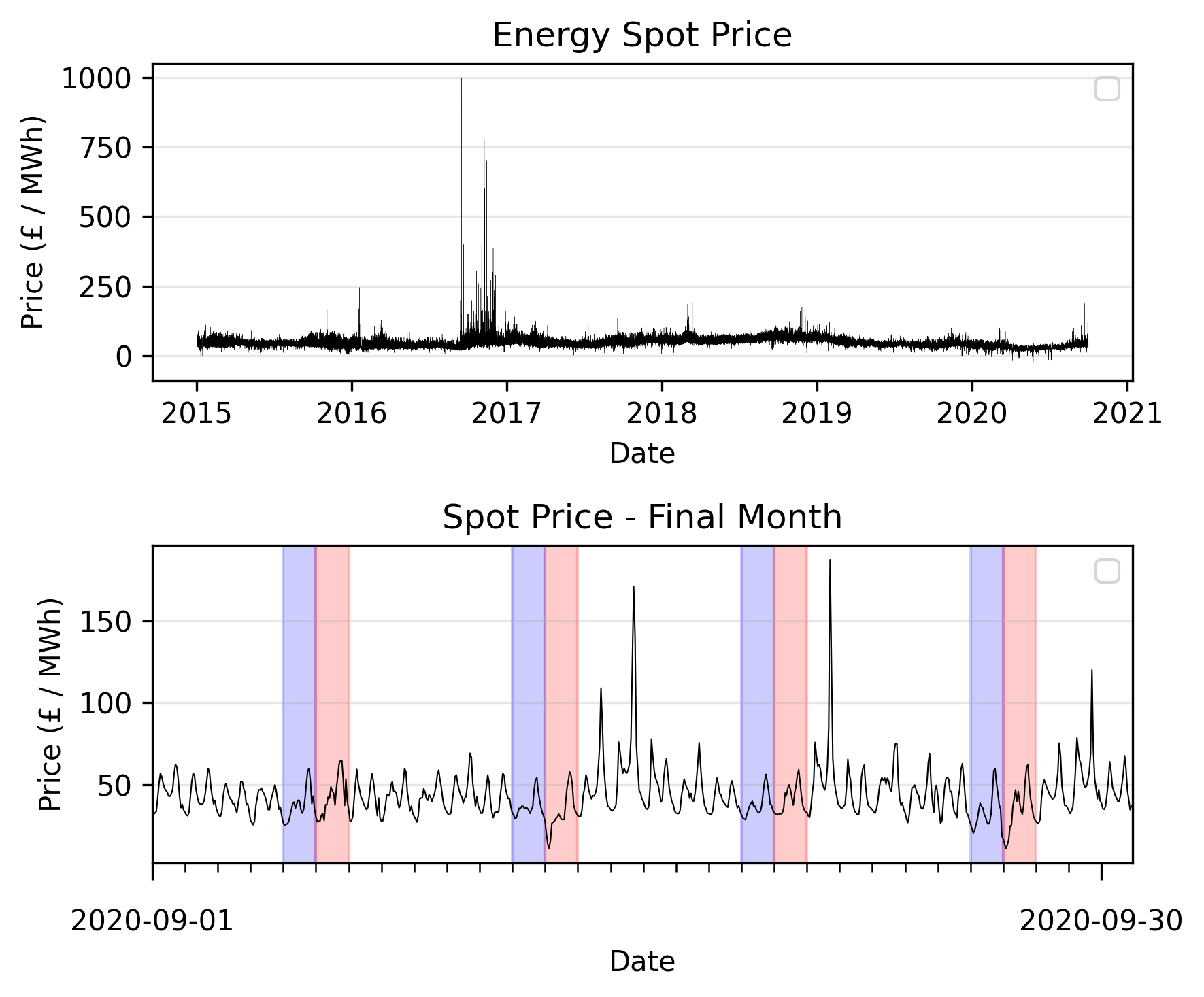
| Figure 1: Spot Price Data. (Top): The hourly-spot price for the training dataset. (Bottom): The hourly spot-price for the validation dataset, the final month of data. The coloured bands highlight weeked spot-prices, purple showing Saturday and pink Sunday. |
|---|
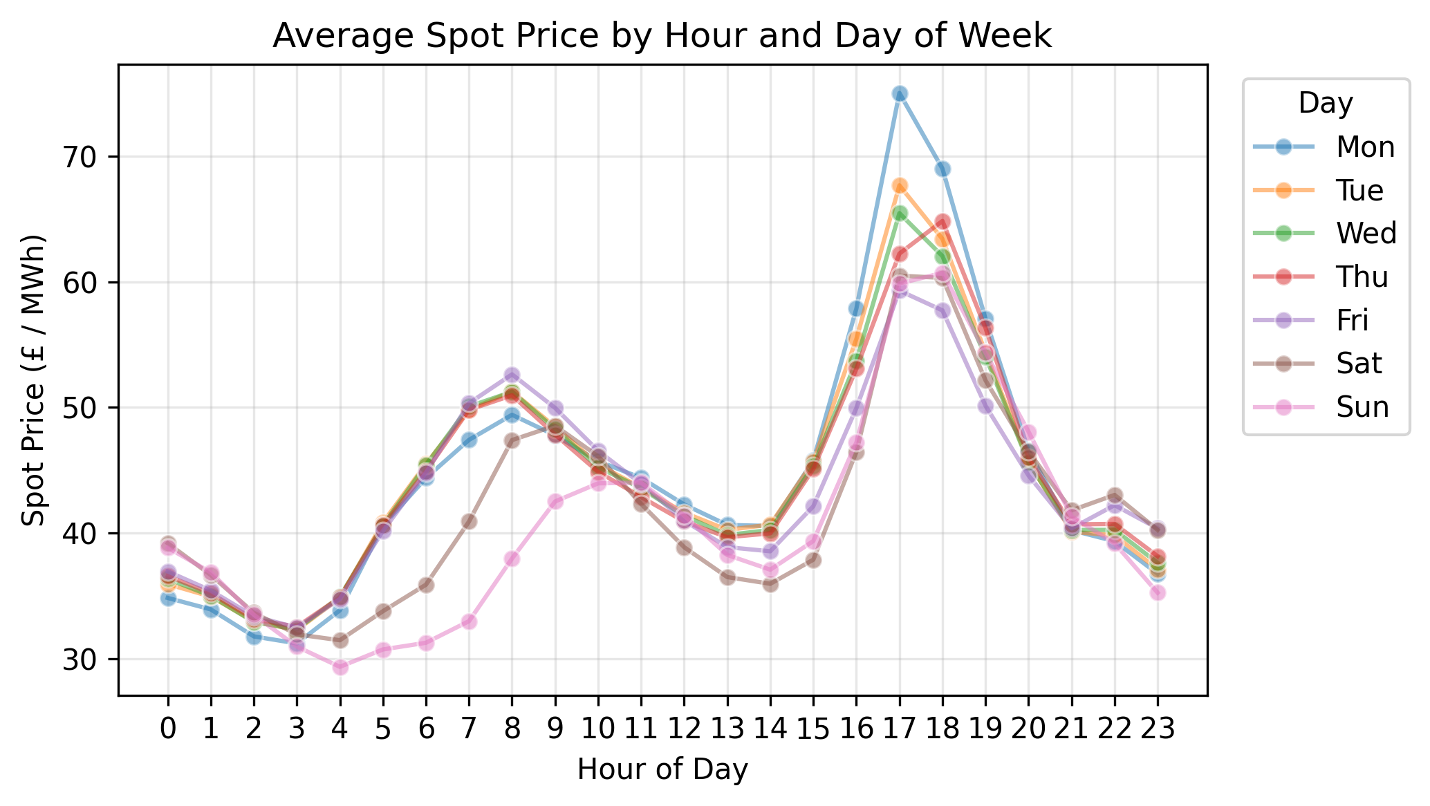
| Figure 2: Average Spot Price is Correlated Between Days. The mean spot price at each hour, separated by day of the week, calculated from the whole dataset. Each colour corresponds to a different day of the week. |
|---|
Methods
Three model categories are compared, each one is considered with and without the use of explanatory (exogenous) variables, and their predictive performance is compared using a sliding window prediction. The energy spot-price is set in 24 hour chucks, that is, the hourly spot prices for tomorrow, for example, are set today. Making predictions 24 hours ahead replicates the real-world need for predicting hourly spot-prices the day before. The dataset is split into two subsets: training and validation, with the final month’s worth of data being used to validate and compare model predictions. A sliding window is used to make predictions, reflecting the necessity to forecast the next day’s energy prices. For each model, the window used spans two years (assumed to be 730 days). Although not shown here, fitting the model on the log-scale provides a better fit to the data and is consistent with other works modelling energy prices, and so all models considered here are on the log-scale. All scripts related to the work presented here can be found in the GitHub repository.
For the models described here, the response variable, $Y_t$, denotes the log spot-price at time $t$. The set of observed exogenous variables observed at time $t$ is denoted $\boldsymbol{x}_{t}$. This set contains the wind and solar generation of the previous day, the forecasted energy load, and two dummy variables indicating whether the observation is made on a Saturday or Sunday. The previous days’ wind and solar generation must be used as generation at the time of spot-price would not be known.
In the remainder of this section, the different models are described, and their implementation is briefly described. A detailed description of each model and its mathematical and statistical underpinnings is not provided here, but a short description is provided.
ARIMA
Auto-Regression Integrated Moving Average (ARIMA) models are ubiquitous within time-series modelling and combine two modelling techniques into a single model. An ARIMA model models the observed value at time $t$ as a linear combination of previously observed values and lags. Crucially, the model assumes that errors are independently distributed with a constant variance (volatility). ARIMA models can also include the effects of seasonality by multiplicatively incorporating a second ARIMA model with a specified seasonal lag. The general form of the model is defined as,
Model fitting
Here, two versions of the seasonal ARIMA (sARIMA) model are investigated, both with and without the inclusion of exogenous variables. The first models the log spot-price, $Y_t$, as a single time-series. The second models each hour as a separate and independent time-series model, essentially fitting 24 independent sARIMA models to the hourly spot-price data. Henceforth, this model will be referred to as sARIMAt. The strong correlation in hourly price, as seen earlier, suggests that this may be a more practical approach than the former.
For each model, the fitting process follows the same steps. Firstly, the model orders are determined. This is a computationally intensive task and requires models with differing orders to be compared via their model fit. Due to computational constraints, a subset of the training data was used, the final 100 days of the training set. Once the model orders are determined, by comparison of the Akaike information criteria (AIC), model predictions for the validation dataset were made via a sliding window using two years of data to predict the next 24 observations (one day’s worth of data).
The seasonal order of the models is not inferred but fixed. During initial inspection of the data, a strong correlation was seen in the hour-specific energy price. As such, a daily seasonality is imposed for the sARIMA models. The hour-specific ARIMAX model will include daily effects within its non-seasonal component, and so a weekly seasonal effect is imposed for this model. Model parameters are inferred via maximum likelihood estimation using the auto_arima and SARIMAX functions in Python. The SARIMAX function is used to make out-of-sample predictions (forecasts).
Seasonal ARIMA and Seasonal ARIMAX
The general form of the seasonal ARIMAX model is given above, and so a formal definition is not necessary here. The mathematical definition of the seasonal ARIMA is found by removing the exogenous variables from the ARIMAX definition, and, again, a formal definition is omitted.
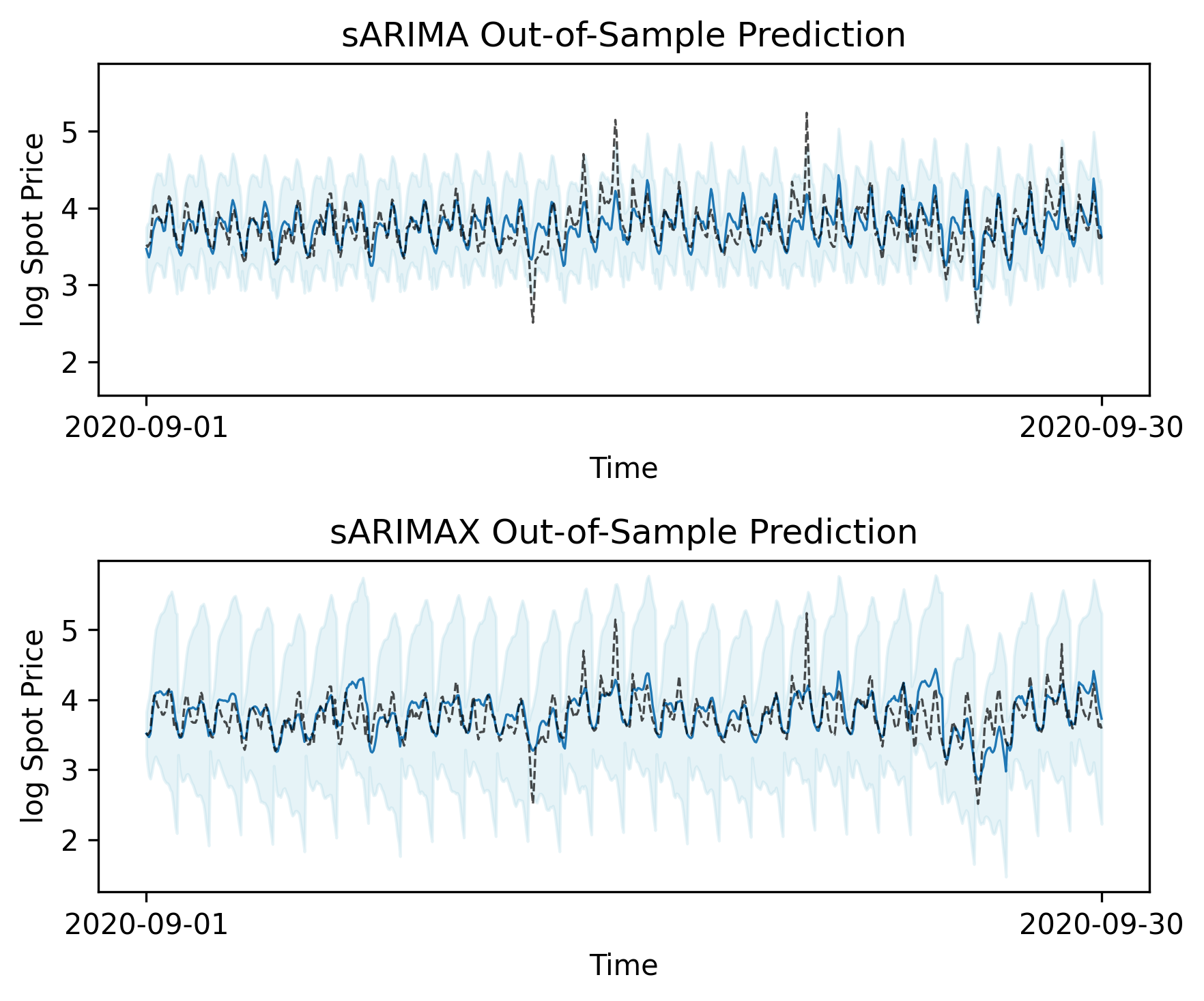
| Figure 3: sARIMA-type Models Out-of-Sample Prediction. The expected value (blue line) and 95% confidence interval (light blue shaded region) for the validation data set, using a two-year sliding window to predict the next 24-hour period under the two sARIMA-type models, which fit seasonal ARIMA models to the log spot-price. The observed log data is shown as a black dashed line. |
|---|
Hourly independence seasonal ARIMA
The hourly-independent model, sARIMAt, differs slightly in its form, where observations made on different hours are assumed to be from an hour-specific seasonal ARIMA model. Let $Y_{t,h}$ be the logged energy spot-price on the $t$-th day and $h$-th hour. It is assumed that each model has the same seasonal effect; however, the orders, $p,d,q,P,D,Q$, are allowed to vary. The model is defined as
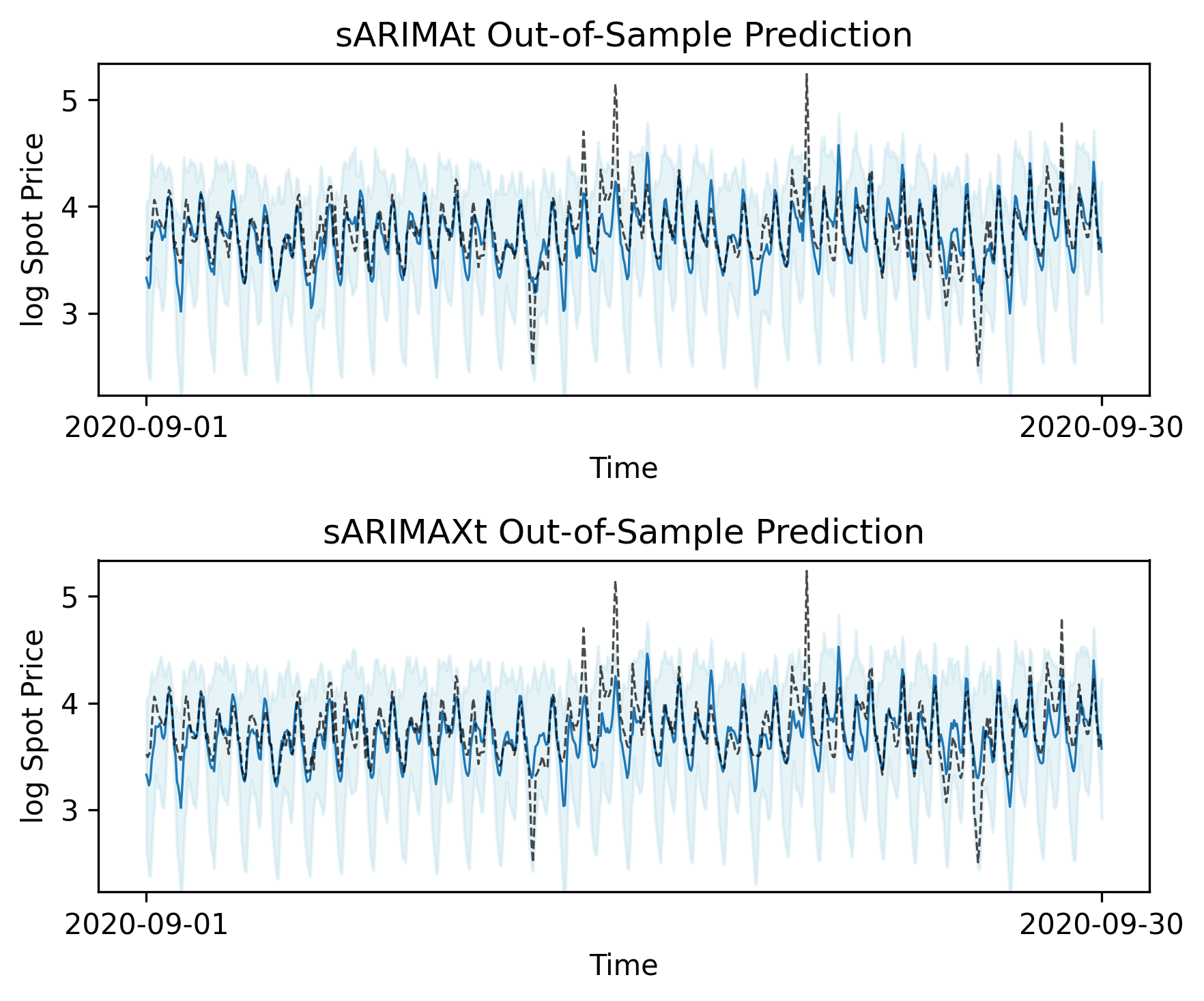
| Figure 4: sARIMAt-type Models Out-of-Sample Prediction. The expected value (blue line) and 95% confidence interval (light blue shaded region) for the validation data set, using a two-year sliding window to predict the next 24-hour period under the two sARIMAt-type models, which fit independent sARIMA models to hour-specific time-series of log spot-price. The observed log data (spot price) is shown as a black dashed line. |
|---|
VAR
The sARIMA model presented considers energy prices as a single univariate time-series. However, the process could be viewed in a multivariate context where energy prices over a single day are treated as a random vector. This also reflects the modelling situation of energy spot-prices, where a single 24-hour period is forecasted. Multivariate extensions of the ARIMA model exist; however, these are notoriously difficult to fit due, in part, to the increased number of model parameters, which scales quadratically with the number of lags, compared to linearly in the univariate setting. Much like the univariate case, the vector autoregressive (VAR) model assumes the current state depends on a linear combination of past states up to a defined lag, $p$. Let $\boldsymbol{Y}_{t}$ be a $k$-dimensional vector of log spot-prices for the $t$-th day i.e. $k=24$, the model is defined as
Where $\boldsymbol{\epsilon}_{t}$ are independent and identically distributed multivariate normal random variables with zero-vector mean and covariance matrix $\Sigma$, and $A_i$ are $k\times k$ coefficient matrices. Exogenous variables are also introduced additively, for a $k\times m$ observed data matrix, the $k\times m$ coefficient matrix is denoted $B$. Similar to ARIMA models, the VAR models assume that volatility is constant. The VAR model is fitted to the logged spot-price data both with and without the inclusion of the exogenous variables.
Model Fit
The VAR models are fitted using the VAR function from the Python statsmodels.tsa.api module. This function also produces the forecasts, which can be seen in Figure 4.
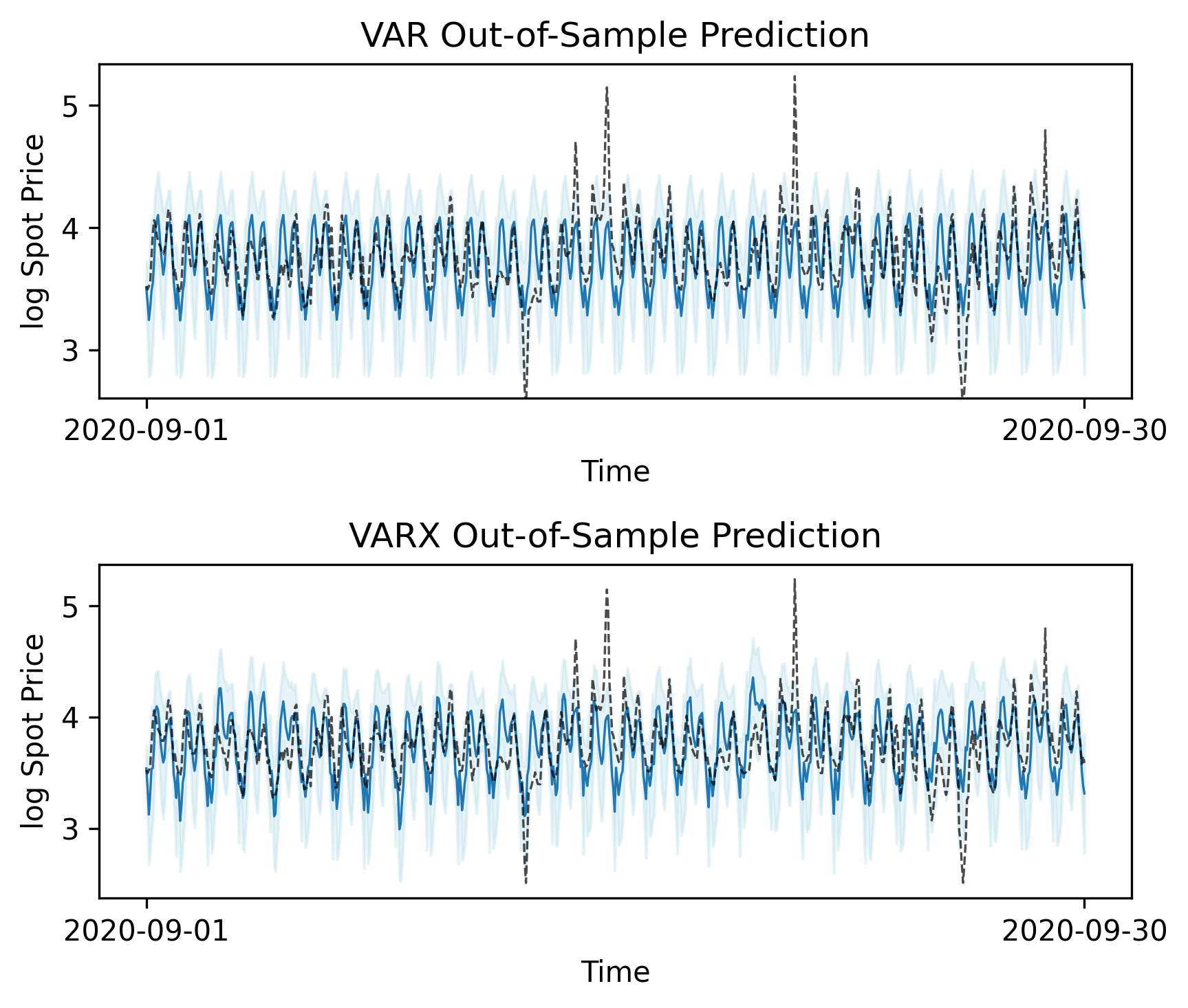
| Figure 5: VAR-type Models Out-of-Sample Prediction. The expected value (blue line) and 95% confidence interval (light blue shaded region) for the validation data set, using a two-year sliding window to predict the next 24-hour period under the two VAR-type models described. The observed log data (spot price) is shown as a black dashed line. |
|---|
GARCH
The ARIMA- and VAR-type models assume that volatility is constant, but this is likely not the case. Spikes in energy prices are known to occur due to a variety of political or practical factors; by their definition, the spikes are outside of the expected range under normal conditions and violate the constant volatility assumption. Generalised autoregressive conditional heteroskedasticity (GARCH) models assume that the volatility is stochastic and dependent on a linear combination of the previous model errors and previous volatilities. A standard GARCH model assumes that the expected value of the time-series is constant. However, it can be extended by introducing methods to model the expected value. Several mean models exist, and here we implement the AR mean model and also its extension to allow for the exogenous variables.
GARCH-ARX
Continuing the notation from the discussion on sARIMA-type models, the GARCH-ARX model is
Model Fitting
The orders of the GARCH-AR models are chosen by fitting a range of models to the training dataset and choosing the parameter set which minimises the AIC. For the AR component, a range of orders are tested, which combine standard and seasonal lags, a seasonal lag of 24 is assumed. The forecasted values and confidence intervals for this model are shown in Figure 6. It can be seen here that the model volatility is dynamic, unlike the previous models discussed, as the confidence intervals are not uniform in size. This is particularly evident for the GARCH-ARX model, where following a spike in spot price, the confidence in the next day’s spot-price descreaces and the confidence intervals widen.
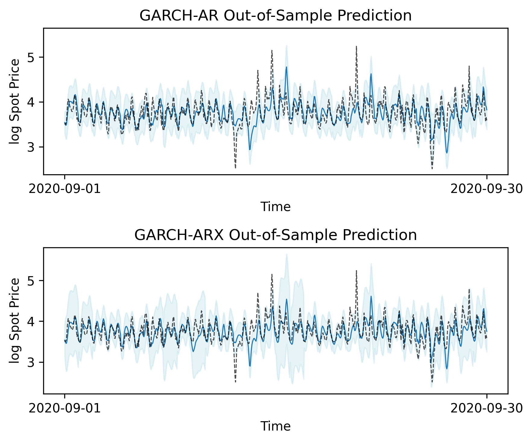
| Figure 6: GARCH-type Models Out-of-Sample Prediction. The expected value (blue line) and 95% confidence interval (light blue shaded region) for the validation data set, using a two-year sliding window to predict the next 24-hour period under the two VAR-type models described. The observed log data (spot price) is shown as a black dashed line. |
|---|
Results
Model fit and predictive performance
To choose the most appropriate model for energy spot-prices two aspects are considered: within-sample model fit and predictive power. To compare within-sample model fit, the log-likelihood is reported in conjunction with the AIC. The AIC measures model fit and complexity, favouring simpler models with fewer parameters. In addition, the mean absolute error (MAE) and root mean squared error (RMSE) between the fitted values (expected values) and observations are reported in Table 1.
It is clear from the AIC statistics that the sARIMA- and GARCH-type models are preferred over the sARIMAt and VAR, showing drastically lower AICs. The difference in their values is due to the increase in estimated model parameters, as seen in the maximised log-likelihood, $\hat{\ell}$, and AIC penalisation of complexity. Recall that the VAR models have a large number of parameters, requiring a $24\times 24$ coefficient matrix at each lag. Similarly, the sARIMAt fit independent sARIMA-type models to the hourly-specific data, approximately increasing the number of parameters by a factor of 24 compared to the sARIMA and sARIMAX models. The GARCH-ARX model results in the lowest AIC, suggesting that this model provides the best compromise between model complexity and fit.
The MAE and RMSE suggest that the sARIMA model provides the best fit to the data, and, interestingly, the same measures suggest that the sARIMAX model has one of the worst. The reduction in model fit after adding exogenous variables could be due to a number of causes. One assumption of the model is that the exogenous variables are uncorrelated to previous observations or errors, which may be violated here as weather is likely correlated with previous observations due to its inherent seasonality. The VAR-type models have the highest RMSE statistics but MAE statistics that are comparable to other models, suggesting that these models have more extreme errors.
The low-AIC and reasonable model fit of the GARCH-type models suggest that the dynamic volatility is a better suited to the data when compared to constant volatility models. The higher MAE and RMSE for the GARCH-type models, compared to the sARIMA model, are likely due to its simpler mean-model, which is less able to model the complex seasonality of spot prices.
| Model | sARIMA | sARIMAX | sARIMAt | sARIMAXt | VAR | VARX | GARCH-AR | GARCH-ARX |
|---|---|---|---|---|---|---|---|---|
| $\hat{\ell}$ | 29800 | 24600 | -620 | -1810 | 45700 | 46700 | 33200 | 34300 |
| AIC | -59500 | -49200 | 1480 | 3830 | -108 | -107 | -66300 | -68500 |
| MAE | 0.0776 | 0.143 | 0.125 | 0.127 | 0.129 | 0.126 | 0.105 | 0.101 |
| RMSE | 0.133 | 0.273 | 0.250 | 0.253 | 0.337 | 0.335 | 0.202 | 0.195 |
Table 1: Within-sample model fit. The Akaike information criteria (AIC), mean absolute error (MAE) of the fitted to observed values, and the root mean square error (RMSE) of the fitted to observed values.
The predictive power of the models tested is summarised in Table 2, where the out-of-sample MAE and RMSE statistics are given. From these statistics, the sARIMA and sARIMAt models provided the greatest predictive power with approximately the same errors. The VAR models diverge the most from their within-sample to out-of-sample model fit, possibly indicating over-fitting. This is likely caused by the large number of parameters, which is reflected in the high AIC statistics in Table 1. The GARCH-type models appear to have a relatively weak predictive power, compared to the sARIMA-type, which is likely due to their simpler mean-model.
| Model | sARIMA | sARIMAX | sARIMAt | sARIMAXt | VAR | VARX | GARCH-AR | GARCH-ARX |
|---|---|---|---|---|---|---|---|---|
| MAE | 0.136 | 0.159 | 0.135 | 0.149 | 0.181 | 0.197 | 0.177 | 0.175 |
| RMSE | 0.185 | 0.220 | 0.186 | 0.203 | 0.240 | 0.258 | 0.246 | 0.243 |
Table 2: Out-of-sample model fit. The Akaike information criteria (AIC), mean absolute error (MAE) of the fitted to observed values, and the root mean square error (RMSE) of the fitted to observed values.
Model assumptions
The models used above come with associated assumptions. Notably, the ARIMA- and VAR-type models assume that residuals are independently and identically distributed by a normal distribution with a constant variance. This assumption should be inspected to give a fuller picture of model fit. The standardised model residuals of the sARIMA model, which showed the lowest within-sample MAE and RMSE, are shown in Figure 6, as well as a QQ-plot of residuals. If volatility is constant, the distribution of the standardised residuals should strongly resemble that of the standard normal distribution, one with zero mean and unit variance, and the points on the QQ-plot should fall close to the diagonal line. This is not the case, the standardised residuals show fatter tails compared to what would be expected, as seen in the divergence from the diagonal line in the extremes. The violation of this assumption indicates that the resulting standard errors are likely wrong, impacting the trustworthiness of confidence intervals for parameter values, fitted values and predicted values. The same, non-constant variance issue appears for all sARIMA- and VAR-type models, although the output is omitted for brevity.
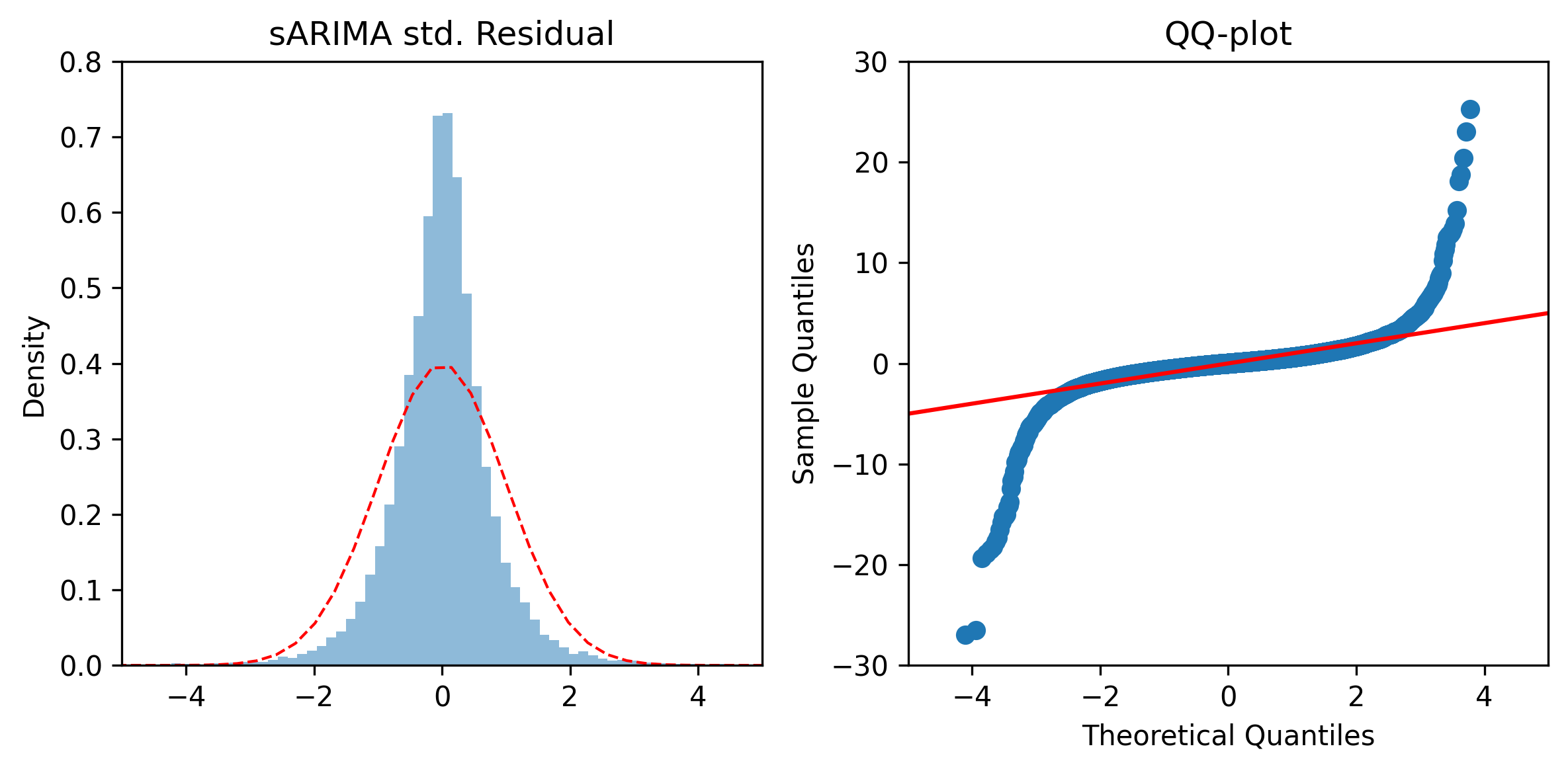
| Figure 7: Standardised Residuals of the sARIMA Model Show Non-Normality. The standardised residuals after fitting the sARIMA model to the training dataset (lightblue histogram). The probability density function of the standard normal distribution. |
|---|
The GARCH-type models assume errors are independently normally distributed with a time-varying variance. The distribution of standardised residuals and QQ-plot can be seen in Figure 8. Residuals are much more in agreement with the modelling assumptions compared to the sARIMA model. However, still show slightly thicker tails than would be expected.
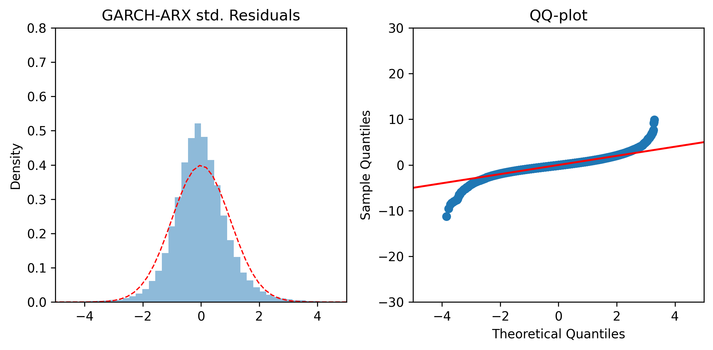
| Figure 8: Standardised Residuals of the GARCH-ARX Model Show Normality. The expected value (blue line) and 95% confidence interval (light blue shaded region) for the validation data set, using a two-year sliding window to predict the next 24-hour period under the two VAR-type models described. The observed log data (spot price) is shown as a black dashed line. |
|---|
Conclusion
From the range of statistical models tested, the sARIMA with no exogenous variables showed the lowest within- and out-of-sample errors, suggesting that this model captured the data the best. However, the data did not conform to one of the ARIMA modelling assumptions, namely, constant volatility. Although the model captured the trend in the data well, due to this failure, the model’s predictive and confidence intervals should not be trusted. Accurately quantifying predictive confidence intervals may be of importance when considering risk management. Hence, despite their improved predictive accuracy, the sARIMA model may not of practical use in situations such as option pricing. The dynamic volatility of the GARCH-type models were well suited to the data and did not show strong violations of the modelling assumptions. However, the forecasts were less accurate than the sARIMA models, indicating that the inclusion of dynamic volatility is important for uncertainty quantification, but the simple AR mean-model used in GARCH-type models is not complex enough to capture the seasonal trends of the spot-prices.
The models may be further improved by the incorporation of other exogenous variables, which may be correlated to spot-price and, importantly, spot-price spikes. Variables such as weather predictions, which would strongly correlate to renewable energy production and thus the marginal spot-price, may be beneficial.
A key drawback to the models used here is that they all considered spot-prices within a price spike to be a part of the same model as those within a normal range, despite them showing very different characteristics. To continue this analysis, it would be interesting to use mixture models or regime-switching models, which are better equipped to handle these distinct states within the data. Another avenue to pursue would be to develop a more accurate mean-model in conjunction with a dynamic volatility seen in the GARCH-type models. Lastly, the data show irratic random behviour which statistical models, such as those seen here, would not be able to capture. Stochastic models are commonly used in finance and could be use here.