Introduction
Electricity differs from many financial and commodity assets because large-scale storage remains expensive, requiring continuous balancing of supply and demand. In the UK day-ahead market, hourly electricity prices are determined through auctions that incorporate expected generation and demand, as well as transmission constraints. In Great Britain, this balance is overseen by the National Energy System Operator (NESO), which manages the grid through a combination of forward markets and a real-time Balancing Mechanism. A key feature of the UK energy market is the day-ahead auction, which is facilitated by two exchanges: EPEX SPOT and Nord Pool’s N2EX.
Accurately forecasting the energy spot price is, therefore, of interest to both energy producers and users. Producers could increase supply if energy prices rise to a sufficient amount, or equally reduce supply when the spot price is too low. Similarly, large-scale energy users could shift intense energy usage to periods of lower prices. In recent years, forecasting energy spot prices has grown considerably more challenging, as the UK’s renewable energy production has increased drastically. The weather-dependent nature of renewable production means that energy production can drop or spike unexpectedly, causing a spike in spot price. Unexpectedly high renewable output can cause prices to drop, and even go negative; similarly, unexpected drops in renewable output can cause prices to spike as more expensive gas and coal are required to cover the shortfall.
This blog continues the investigation of modelling energy spot prices within Great Britain from my previous posts. The aim of this blog differs to others, which were focused on model comparison, and we look at a practical inference scheme for streaming data. Streaming data refers to data which arises sequentially, and we consider how to update parameter beliefs as new observations are available in real-time. Energy spot prices are an natural example of streaming data because observations arrive continuously and parameter beliefs must be updated in real time for price forecasting, derivative pricing and risk management. Adding to this, parameter beliefs may not be well reflected by a static distribution as external factors impact energy price dynamics, and parameter beliefs must be updated to reflect this.
Methods
The data
The data is sourced from Transmission System Operators and power exchanges, and is available through kaggle. A detailed description of collection methods and data structure is given on a GitHub page. The dataset is large, containing observed spot prices in many regions and a range of explanatory variables. Here, we restrict the dataset to hourly energy spot-prices determined on the day-ahead auction. The data, however, contains some missing values, which are filled using a smoothed Kalman filter when modelling begins, to avoid added difficulties of missingness during parameter inference. In this blog, we consider a single model of energy spot price, and implement an online Bayesian inference to infer its parameters.
The model
Energy spot price, $S_t$, is modelled by additively combining a deterministic mean function, $\Lambda_t$, and a stochastic component, $X_t$, to capture the seasonal trend and random fluctuations, respectively. The model can therefore be written as $$ S_t = \Lambda_t + X_t, $$ where $t$ indicates time. The spot price is measured hourly, and this is the time scale we consider the model on. The seasonal trend is considered to be a linear combination of categorical variables indicating the hour of the day and the day week, $$ \Lambda_t = \mu_0 + \frac{\mu_1}{8760} t + \beta_{A_t} + \gamma_{B_t}, $$ where $t$ is the time, in years.
The stochastic component is modelled as an Ornstein-Uhlenbeck process with a stochastic volatility, modelled by an independent Ornstein-Uhlenbeck process on the log-scale. Such models are commonly used in derivatives pricing, and can be written as $$ dX_t = -\theta X_t,dt + \sigma_t,dW_t^X, $$ $$ dV_t = \theta_v (\mu_v - V_t),dt + \sigma_v,dW_t^V, $$ $$ \sigma_t = \exp(V_t). $$
Stochastic volatility models are common when considering energy prices, which characteristically display non-constant volatility, periods of increased volatility, known as volatility clusters, and thick tails in price density. The volatility model here is an Ornstein-Uhlenbeck process, which is a mean-reverting process and assumes the volatility will return to some long-term mean, $\mu_v$, but allows stochastic deviations from this. The stochastic variable $X_t$ is a zero-mean reverting process, allowing the spot price model to return to the deterministic mean function.
The Ornstein-Uhlenbeck process has a closed-form transition density, allowing the conditional likelihood to be calculated exactly. Using that the volatility is constant in the interval $[t, t+\Delta t)$, the transition density is $$ S_{t+1} \mid S_t \sim \mathcal{N}!\left(\Lambda_{t+1} + \alpha (S_t - \Lambda_t),; \frac{\sigma_t^2}{2\theta}(1 - \alpha^2) \right) $$ $$ \alpha = e^{-\theta}. $$
Inference Scheme
The unobserved (latent) volatility process, $V_t$, complicates inference by making the marginal observed-data likelihood, $p(S_{0:t}|\boldsymbol{\theta})$, hard to evaluate. Inference may proceed by implenting the sequential Monte Carlo squared (SMC$^2$), which approximates the posterior distribution, $p(\boldsymbol{\theta} | S_{1:t})$, by a empirical distribution of parameter particles, ${(\boldsymbol{\theta}^{(i)}, u_i)}_{i=1}^N$, where $u_i$ is the probability of particle $\boldsymbol{\theta}^{(i)}$. Each particle is associated with a “cloud” of $M$ latent-state particles, $V_t^{i,1:M}$, which allow the unbiased estimation of the observed-data likelihood, $p(S_t | \boldsymbol{\theta}^{(i)})$, by the particle filtering algorithm. For each new observation parameter weights, $u_i$, are updated using by the estimated likelihood.
Such schemes are known to suffer from degeneracy, where the cloud of parameter particles collapses to a few values with a high likelihood. Degeneracy prohibits exploration of the parameter space, leading to poor parameter estimates. To overcome this, a particle rejuvenation scheme is implemented, which updates parameter particles when the effective sample size (ESS) of the set drops below a chosen value. Here, the particles are updated by a Metropolis-Hastings (MH) step, which targets the joint posterior distribution. The MH step requires calculation of the model likelihood to evaluate an acceptance probability, which, again, can be estimated via a particle filter.
The inference scheme was implemented in Python 3.13, the scripts for which can be found in the GitHub repo. The scheme was implemented with $M=2000$ latent state particles per $N=1000$ parameter particles. The number of particles meant computational cost is significant, and care was taken to implement scripts which are efficient, utilising independence between calculations and the particle-cloud nature of the scheme to vectorise calculations wherever possible. To infer hourly and daily effects the zero-constraint was imposed, setting $\beta_1 = \gamma_1 = 0.0$, resulting in a total of 35 unknown parameters. To improve exploration of the high-dimensional parameter space, a blockwise MH update was implemented, each using a normal random-walk proposal distribution. Five parameter blocks were considered; hourly effects were separated into three blocks, daily effects, and the remaining parameters. The covariance matrix of the proposal distributions is set to $\frac{2.34^2}{ n_{\theta_j}} \widehat{\text{Var}}(\boldsymbol{\theta_j})$, where $n_{\theta_j}$ is the number of parameters in the block and $\widehat{\text{Var}}(\boldsymbol{\theta_j})$ is the sample covariance from previous set of parameter particles. The rejuventation step was triggered if the effective sample size of the particle parameters dropped below $0.5M$. All calculations of the likelihood, particle probabilities, and acceptance probabilities were done on the log scale for numerical stability; similarly, log-sum-exp stabilisation was implemented. The inference for parameters: $\theta, \theta_v,$ and $\sigma_v$, was done on the log-scale, as these parameters are constrained to be positive this removed issues associated with zero density and improved exploration of the parameter space for small values. Prior distributions were kept relatively vague, reflecting the lack of prior information, exact specificvations can be found in the GitHub repo.
Compared to batch inference, which would independently infer parameter values and latent states from scratch with each new observation, the SMC$^2$ algorithm is very efficient, with a (somewhat) fixed number of computations per update. The somewhat caveat was added due to the rejuvenation step which is not guaranteed to occur at each update. The computational cost of rejuvenation also grows approximately linearly with the number of observations, as the MH step requires estimation of the observed-data likelihood via particle filter for data up until the current time point. However, this addition should be negligible compared to the computational cost of batch inference. Another advantage of the SMC$^2$ algorithm is that the storage cost of each update is approximately constant, which is a key advantage as the dataset size grows; it is only necessary to store the previous iterations’ clouds of parameter and latent particles, and estimated likelihoods per parameter particle. A detailed introduction to particle filtering and sequential Monte Carlo methods can be found here.
Results
Applying SMC$^2$ retrospectively to a fixed dataset is computationally more expensive than a batch inference scheme such as Stan. Its advantage lies instead in sequential updating as new observations arrive. As a consequence, the training dataset was constrained to seven days of hourly spot prices (168 observations) from the last week of August 2020. Nevertheless, the scheme was able to update beliefs a posteriori for parameters of the models stochastic component and most of the parameters of the deterministic mean function. The accuracy of the SMC$^2$ can be inspected by comparing posterior distributions to those generated by Stan. This may be done in numerous ways; here, we compare the distributions of posterior differences for each parameter and check whether zero lies outside the associated 95% credible interval, checking for a substantial difference in the parameter’s value. No parameter shows a substantial difference in value between inference schemes, Table 1 shows the expected values of the posterior differences for a subset of parameters and their credible intervals.
| $\text{E}[\Delta \theta]$ | 95% CI | |
|---|---|---|
| $\log \theta $ | 0.383403 | $(-0.470, 1.34)$ |
| $ \mu_v $ | 0.058987 | $(-0.345, 0.490)$ |
| $\log \theta_v$ | 0.067769 | $(-1.41, 1.30)$ |
| $\log \sigma_v$ | 0.047217 | $(-0.624, 0.676)$ |
| Table 1: Posterior difference distributions between SMC$^2$ and Stan. The expected postesterior difference and 95% credible intervals for the four the parameters of the models stochastic component. |
|---|
The one-step-ahead posterior credible intervals for the spot price and the inferred latent volatility process can be seen in Figure 1. The inferred volatility appears to match the process well, spiking in the same regions which show spot-price spikes, specifically for the large spot-price peaks around days two and three of those shown in the figure. Initially, the posterior distributions are dominated by vague prior beliefs, resulting in vague posterior predictive distributions, but after only a few observations, this uncertainty reduces and the predictions for both the spot price and volatility reduce to a reasonable degree.
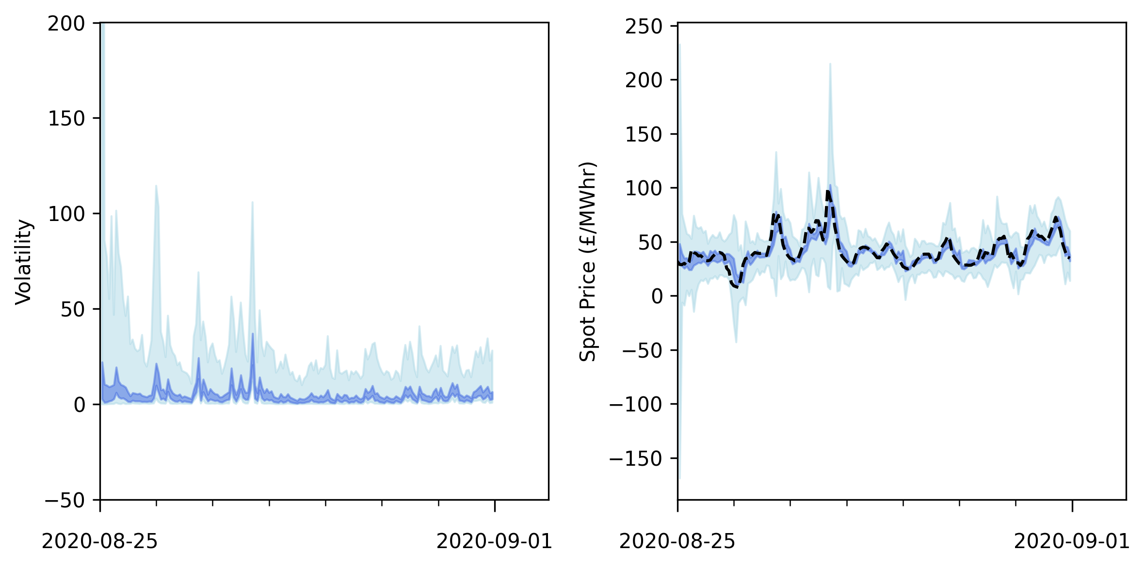
| Figure 1: Posterior Credible Intervals. The posterior 99% (light blue) and 50% (dark blue) credible intervals for the latent volatility process (left) and the one-step-ahead posterior predictive distribution for energy spot price. |
|---|
Online inference of parameters allows us to see how parameter beliefs change in real-time as more data is observed. Figure 2 shows the posterior credibles at each time point for the training dataset. It is clear that in the beginning, when the dataset is small, the prior distribution dominates parameter beliefs. However, with the addition of more data, beliefs are updated and move away from the priors. This is even the case for parameters of the unobserved latent process, which can be difficult to infer due to their unobserved nature. The shrinking credible intervals demonstrate how information accumulates sequentially, and uncertainty declines as more observations become available.
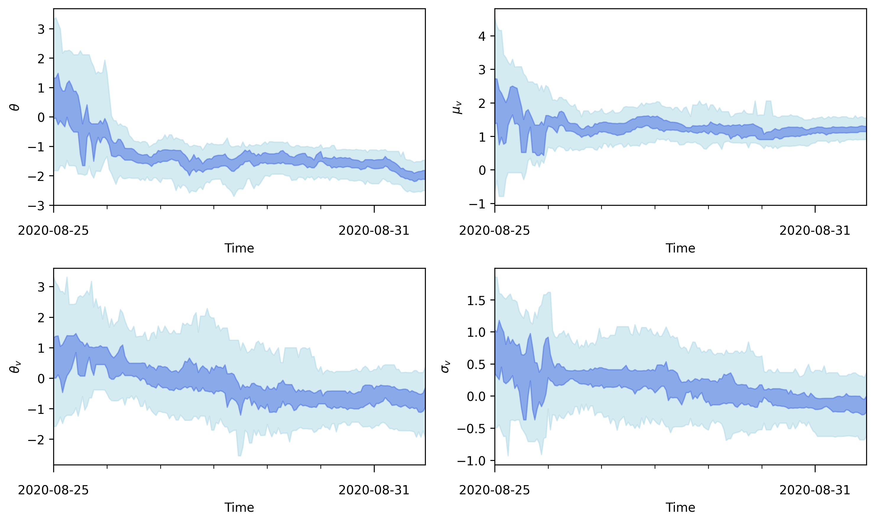
| Figure 2: Parameter Beliefs in Time. The posterior 99% (light blue) and 50% (dark blue) credible intervals after each new observation for the four parameters of the stochastic component of the model. |
|---|
As mentioned, without particle rejuvenation, the computational cost of each update should be approximately constant. However, when a particle rejuvenation step is triggered, a comparatively high cost is incurred, requiring the execution of the particle filter algorithm per parameter proposal of the MH kernel. Further, this cost grows approximately linearly with the number of observations, see Figure 3, which shows computing time for each update of the SMC$^2$ scheme. Timings were conducted on a MacBook Pro with an M2 chip and 16Gb RAM. The MH proposal distribution resulted in average acceptance rates between 0.22 and 0.26 for each block, in line with the generally accepted 0.234 optimal acceptance rate. Particle rejuvenation was triggered 81 times, out of a possible 168, demonstrating a fairly high level of particle degeneracy within the scheme. The MH step can effectively rejuvenate the parameter particle set and increase ESS as seen in Figure 3. Also note that particle rejuvenation was triggered at higher rates when the number of observations is low and appears to reduce in frequency as more observations are made.
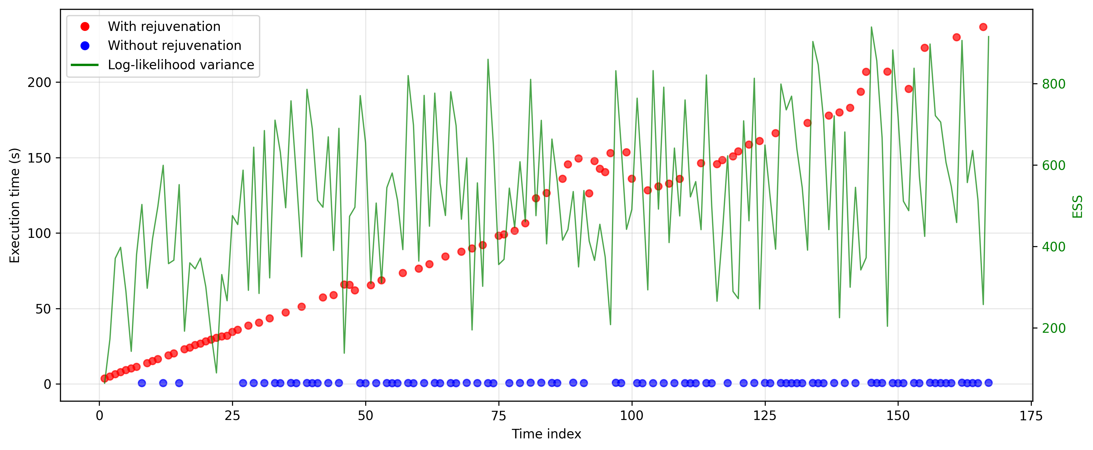
| Figure 3: SMC$^2$ Execution Time. The time required for each iteration of the SMC$^2$ algorithm in seconds (left axis). Updates which triggered a particle rejuvenation step are coloured red otherwise execution times are blue. The ESS (right axis) of the parameter particle set at each time point is shown in green. |
|---|
Conclusion
The SMC$^2$ algorithm provides a scheme which can infer both parameter values and latent states of a stochastic model. The algorithm approximates the posterior distribution by a cloud of weighted parameter particles, which are updated with each new observation, providing real-time online Bayesian inference. The algorithm achieves this by implementing the particle filter algorithm, which estimates the observed data likelihood, to update the parameter particle weights. The parameter particles are known to suffer from degeneracy, a collapse of the posterior estimate to a single point, which can be overcome by particle rejuvenation. Here, particles were rejuvenated by the MH kernel when the effective sample size of the parameter particles dropped below a threshold.
The storage cost of the SMC$^2$ scheme is low, requiring only the cloud of parameters and latent particles to be stored between updates and without a rejuvenation step, the computational cost is minimal and constant. When investigating stochastic models of spot price previously, see here, it was found that the Stans large storage costs were prohibitive to long chains and generating posterior predictives within Stan. This meant shorter chains had to be used, some of which showed signs of non-convergence, and post-inference predictions had to be made in Python.
The MH kernel adds a relatively high computational cost to the algorithm, requiring the estimation of the likelihood for each parameter proposal and thus an execution of the particle filter algorithm for the entire observed dataset. Despite this cost, the scheme offers significant improvements compared to batch inference, which would require executing parameter inference from scratch with each new observation. This is not only wasteful, ignoring information gained from the previous batch of inference, but it can also carry high computational costs.
The SMC$^2$ scheme was successful in parameter and latent state inference, but the computational cost of particle rejuvenation would continue to grow as more data is observed, which may become prohibitive. Therefore, the next steps would be to investigate computational efficiencies, such as parallelisation or translating the inference scheme to a faster programming language such as Julia or C++. Alternatively, other rejuvenation steps could be investigated which do not require the estimation of the observed data likelihood via the particle filtering algorithm, as this is the primary computational burden.
Final Remarks
Online inference schemes can be extremely useful for streaming data, such as energy spot prices, as they can update parameter beliefs and model predictions with each new observation. Here, we showed that parameters of a stochastic volatility model could be inferred by such a scheme and highlighted the computational burdens associated with it.